Probability, Statistics, and Data: A Fresh Approach Using R

Chapter 8 Inference on the Mean

Car accidents are sometimes caused by unintended acceleration, when the driver fails to realize that the car is accelerating in time to apply the brakes. This type of accident seems to happen more with older drivers. Hasegawa, Kimura, and Takeda⁵² developed an experiment to test whether older drivers are less adept at correcting unintended acceleration.

The set-up of the experiment was as follows. Older (65+) drivers and younger (18-32) drivers were recruited. The drivers were put in a simulation and told to apply the brake when a light turned red. Ninety percent of the time, this would work as desired, but ten percent of the time, the brake would instead speed up the car. When the participants became aware of the unintended acceleration, they were to release the center pedal and push the left pedal to stop the acceleration.

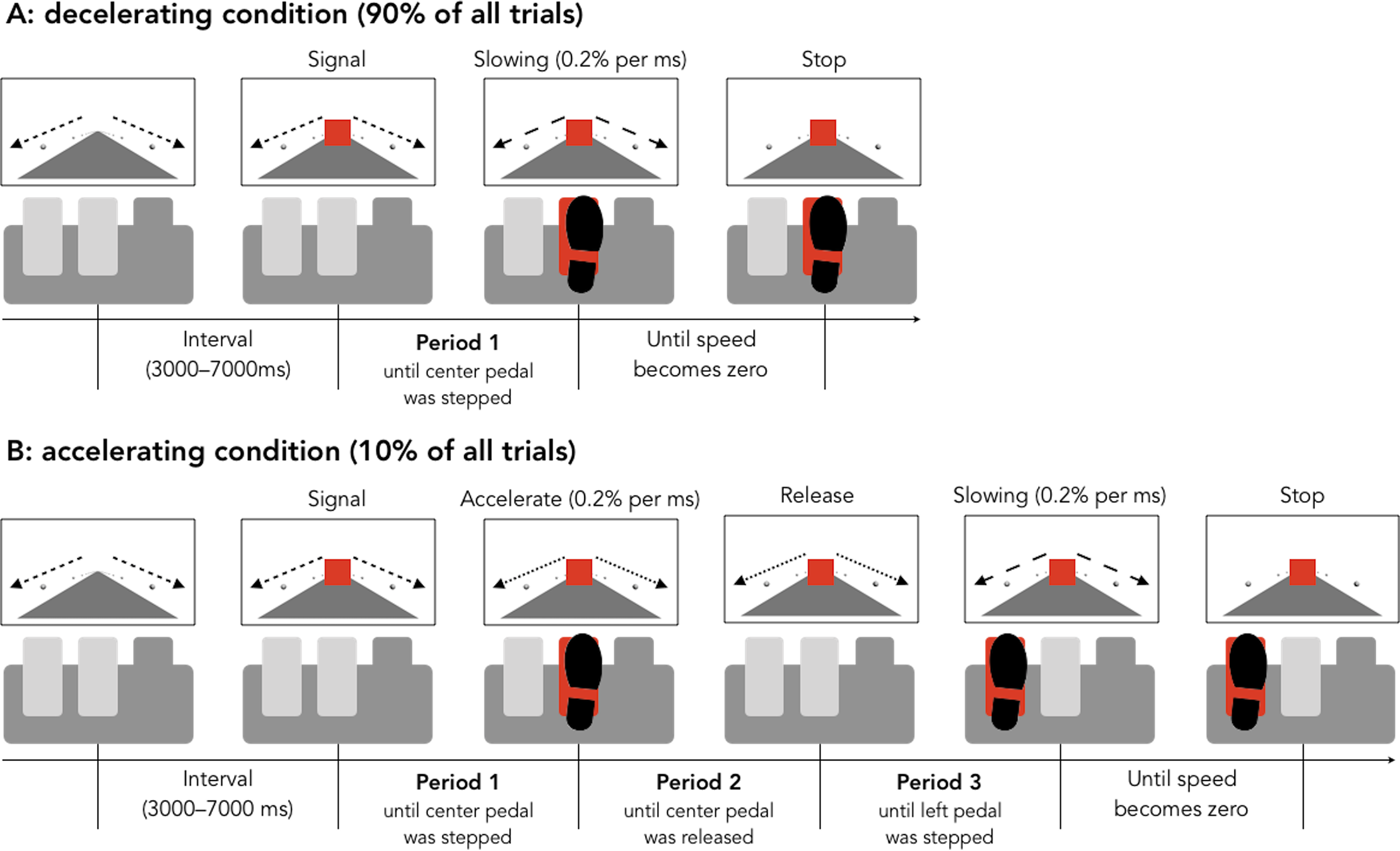
Figure 8.1: Figure from Hasegawa, et al.

Image credit: Hasegawa et al.Image Credit
Hasegawa et al. This is an open access article distributed under the terms of the Creative Commons Attribution License. https://journals.plos.org/plosone/article?id=10.1371/journal.pone.0236053

The data from this experiment is available in the brake data set from the fosdata package.

brake <- fosdata::brake

The authors collected a lot more data than we will be using in this chapter! Let’s focus on the latency (length of time) variables. The experimenters measured three things in the case when the brake pedal activated acceleration:

• latency_p1: The length of time before the initial application of the brake.
• latency_p2: The length of time before the brake was released.
• latency_p3: The length of time before the pedal to the left of the brake was pressed, which would then stop the car.

The experimenters desired to determine whether there is a difference in latency between older and younger drivers in the population of all drivers. The experiment measured a sample of drivers and produced the data shown in the accompanying figure.

brake %>%
  tidyr::pivot_longer(
    cols = matches("^lat"),
    names_to = "type", values_to = "time"
  ) %>%
  ggplot(aes(x = type, y = time, color = age_group)) +
  geom_boxplot()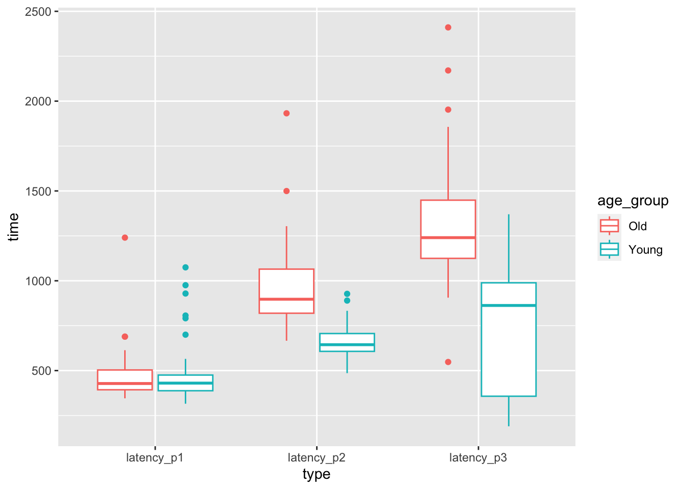

Figure 8.2: Latencies for drivers pressing, releasing, and correcting the pedal of an accelerating car.

At a first glance, it seems like there may not be a difference in time to react to the red light between old and young, but there may well be a difference in the time to realize a mistake has been made. However, there is considerable overlap between the distributions for old and young. Is it possible that the apparent difference is due to the random nature of the sample, rather than a true difference in the population? The purpose of this chapter is to be able to systematically answer such questions through a process known as statistical inference.

Once the theory is developed, we return to this experiment in Example 8.21 and test whether the mean length of time for an older driver to release the pedal after it resulted in an unintended acceleration is the same as the mean length of time for a younger driver.

8.1 Sampling distribution of the sample mean

In Section 5.5 we discussed various sampling distributions for statistics related to a random sample from a population. The \(t\) distribution first described in Section 5.5.2 will play an essential role in this chapter, so we review and expand upon that discussion here. Theorem 5.5 states that if \(X_1,\ldots,X_n\) are iid normal random variables with mean \(\mu\) and standard deviation \(\sigma\), then \[ \frac{\overline{X} - \mu}{S/\sqrt{n}} \] has a \(t\) distribution with \(n - 1\) degrees of freedom, where \(S\) is the sample standard deviation and \(\overline{X}\) is the sample mean. We write this as \[ \frac{\overline{X} - \mu}{S/\sqrt{n}} \sim t_{n - 1}. \] A random variable that has a \(t\) distribution with \(n - 1\) degrees of freedom is said to be a \(t\) random variable with \(n - 1\) degrees of freedom.

Tryit 8.1

Simulate the pdf of \(\frac{\overline{X} - \mu}{S/\sqrt{n}}\) when \(n = 3\), \(\mu = 5\), and \(\sigma = 1\), and compare to the pdf of a \(t\) random variable with 2 degrees of freedom.

Figure 8.3 compares the pdf of \(t\) random variables with various degrees of freedom.

## Warning: Using `size` aesthetic for lines was deprecated in ggplot2 3.4.0.
## ℹ Please use `linewidth` instead.
## This warning is displayed once every 8 hours.
## Call `lifecycle::last_lifecycle_warnings()` to see where this warning was generated.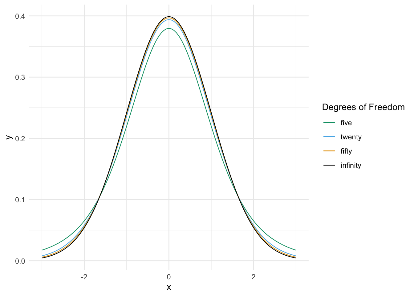

Figure 8.3: Probability density functions of standard normal and \(t\) random variables.

We see from the graphs that \(t\) distributions are bump-shaped and symmetric about 0. For all \(t\) random variables, 0 is the most likely outcome, and the interval \([-k, k]\) has the highest probability of occurring of any interval of length \(2k\).

As the number of degrees of freedom increases, the tails of the \(t\) distribution become lighter. This means that \[ \lim_{M \to \infty} \frac{P(|T_\nu| > M)}{P(|T_\tau| > M)} = \infty \] for \(T_\nu\) and \(T_\tau\) \(t\) random variables with degrees of freedom \(\nu < \tau\).

Thinking of the \(t\) distribution as the sampling distribution of \(\frac{\overline{X} - \mu}{S/\sqrt{n}}\), a smaller value of \(n\) means that \(S\) gives a worse approximation to \(\sigma\), resulting in a distribution that is more spread out. As the sample size goes to \(\infty\), we become more and more sure of our estimate of \(\sigma\), until in the limit the \(t\) distribution is standard normal.

Theorem 8.1

For \(n = 1, 2, \ldots\) let \(T_n\) be a \(t\) random variable with \(n\) degrees of freedom. Let \(Z\) be a standard normal random variable. Then, \[ T_n \to Z \] in the sense that for every \(a < b\), \[ \lim_{n \to \infty} P(a < X_n < b) = P(a < Z < b) \]

The difference between the pdfs of a \(t\) random variable and a standard normal random variable may not appear large in the picture, but it can make a substantial difference in the computation of tail probabilities, as 8.1 explores. The results of statistical inference are especially sensitive to these tail probabilities.

Example 8.1

Let \(T\) be a \(t\) random variable with 3 degrees of freedom, and let \(Z\) be a standard normal random variable. Compare \(P(T < -2.5)\) with \(P(Z < -2.5)\).

On one hand, if we compute the absolute difference between the two probabilities, we get \(\left|P(Z < -2.5) - P(T < -2.5)\right| \approx 0.038\), which may seem small.

pt(-2.5, df = 3) - pnorm(-2.5)

## [1] 0.03764366

On the other hand, if we compute the relative magnitude of the probabilities, we see that \(P(T < -2.5)\) is approximately 7 times larger than \(P(Z < -2.5)\), which is quite a difference!

pt(-2.5, df = 3) / pnorm(-2.5)

## [1] 7.062107

Tryit 8.2

About how many degrees of freedom for a \(t\) random variable \(T\) do you need before \(P(T < -2.5)\) is only 50% larger than \(P(Z < -2.5)\)?

Now suppose that \(X_1, \dotsc, X_n\) represent data which is randomly sampled from a population which is normally distributed with mean \(\mu\) and standard deviation \(\sigma\). We do not know the values of \(\mu\) and \(\sigma\), but we do know that \(\frac{\overline{X} - \mu}{S/\sqrt{n}}\) has the \(t\) distribution with \(n-1\) degrees of freedom.

Let \(t_{\alpha}\) be the unique real number such that \(P(T > t_{\alpha}) = \alpha\), where \(T\) is a \(t\) random variable with \(n-1\) degrees of freedom. Note that \(t_{\alpha}\) depends on \(n\), because the \(t\) distribution has more area in its tails when \(n\) is small.

Then, we know that \[ P\left( t_{1 - \alpha/2} < \frac{\overline{X} - \mu}{S/\sqrt{n}} < t_{\alpha/2}\right) = 1 - \alpha. \]

Because the \(t\) distribution is symmetric, \(t_{1-\alpha/2} = -t_{\alpha/2}\), so we can rewrite the equation symmetrically as:

\[ P\left( -t_{\alpha/2} < \frac{\overline{X} - \mu}{S/\sqrt{n}} < t_{\alpha/2}\right) = 1 - \alpha. \]

Now with probability \(1-\alpha\), \[ -t_{\alpha/2} < \frac{\overline{X} - \mu}{S/\sqrt{n}} < t_{\alpha/2} \] so \[ -t_{\alpha/2}S/\sqrt{n} < \overline{X} - \mu < t_{\alpha/2}S/\sqrt{n}. \] Multiplying through by \(-1\) and then reversing the order of terms, \[ -t_{\alpha/2}S/\sqrt{n} < \mu - \overline{X} < t_{\alpha/2}S/\sqrt{n} \] with probability \(1-\alpha\). Finally, add \(\overline{X}\) to all terms to conclude \[ P\left(\overline{X} - t_{\alpha/2} S/\sqrt{n} < \mu < \overline{X} + t_{\alpha/2} S/\sqrt{n}\right) = 1 - \alpha. \]

Let’s think about what this means. Take \(n = 10\) and \(\alpha = 0.10\) just to be specific. This means that if we were to repeatedly take 10 samples from a normal distribution with fixed mean \(\mu\) and any \(\sigma\), then 90% of the time, \(\mu\) would lie between \(\overline{X} + t_{\alpha/2} S/\sqrt{n}\) and \(\overline{X} - t_{\alpha/2} S/\sqrt{n}\). That sounds like something that we need to double check using a simulation!

t05 <- qt(.05, 9, lower.tail = FALSE)
# Take samples from a normal population with mean 5 and sd 8
mu <- 5
sigma <- 8
mean(replicate(10000, {
  X <- rnorm(10, mu, sigma) # sample of size 10
  Xbar <- mean(X) # sample mean
  SE <- sd(X) / sqrt(10) # standard error
  (Xbar - t05 * SE < mu) & (mu < Xbar + t05 * SE)
}))

## [1] 0.9002

The first line computes \(t_{\alpha/2}\) using qt, the quantile function for the \(t\) distribution, here with 9 degrees of freedom. Then we check the inequality given above. It works; the interval contains the value \(\mu = 5\) about 90% of the time.

Tryit 8.3

Repeat the above simulation with \(n = 20\), \(\mu = 7\), and \(\alpha = .05\).

8.2 Confidence intervals for the mean

In the previous section, we saw that if \(X_1, \ldots, X_n\) is a random sample from a normal population with mean \(\mu\), then \[ P\left(\overline{X} - t_{\alpha/2} S/\sqrt{n} < \mu < \overline{X} + t_{\alpha/2} S/\sqrt{n}\right) = 1 - \alpha. \] This leads naturally to the following definition.

Definition 8.2

Given a sample of size \(n\) from iid normal random variables, the interval

\[ \left( \overline{X} - t_{\alpha/2} S/\sqrt{n},\ \ \overline{X} + t_{\alpha/2} S/\sqrt{n} \right) \]

is a \(100(1 - \alpha)\%\) confidence interval for \(\mu\).

Confidence intervals are random because they depend on the random sample. Sometimes a sample will produce a confidence interval that contains \(\mu\), and sometimes a sample will produce a confidence interval that does not contain \(\mu\). Since \(\mu\) is typically not known when performing experiments, there is typically no way to determine whether a particular confidence interval succeeded in capturing the population mean. However, the procedure of taking a sample and computing a confidence interval will succeed in capturing the population mean \(100(1 - \alpha)\%\) of the time. This is what “confidence” means.

Over all scientific experiments that use confidence intervals to describe population means, we accept the fact that some proportion (\(\alpha\), specifically) will fail to contain the true mean, and we will not know which ones.

Example 8.3

Consider the heart rate and body temperature data normtemp.⁵³

You can read normtemp as follows.

normtemp <- fosdata::normtemp

What kind of data is this?

str(normtemp)

## 'data.frame':    130 obs. of  3 variables:
##  $ temp  : num  96.3 96.7 96.9 97 97.1 97.1 97.1 97.2 97.3 97.4 ...
##  $ gender: int  1 1 1 1 1 1 1 1 1 1 ...
##  $ bpm   : int  70 71 74 80 73 75 82 64 69 70 ...

head(normtemp)

##   temp gender bpm
## 1 96.3      1  70
## 2 96.7      1  71
## 3 96.9      1  74
## 4 97.0      1  80
## 5 97.1      1  73
## 6 97.1      1  75

We see that the data set is 130 observations of body temperature and heart rate. There is also gender information attached, that we will ignore for the purposes of this example.

Let’s visualize the data through a boxplot (turned sideways with coord_flip).

ggplot(normtemp, aes(x = "", y = temp)) +
  geom_boxplot(notch = TRUE) +
  coord_flip()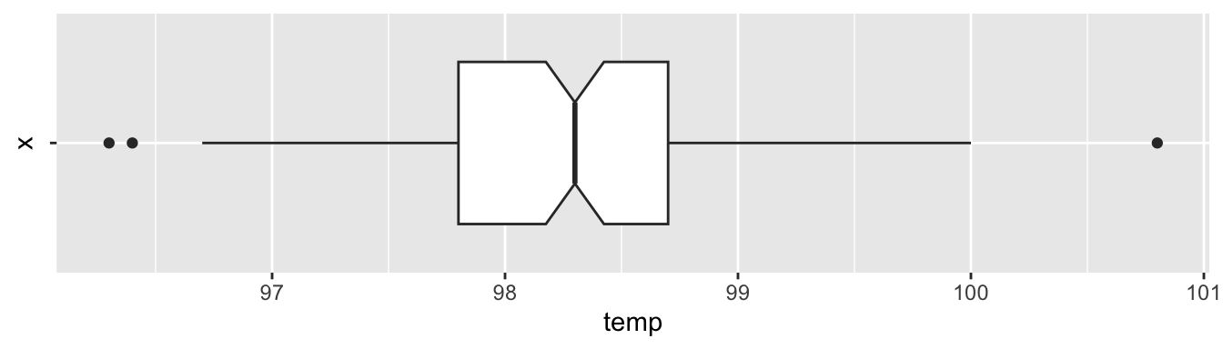

The data looks symmetric without concerning outliers. According to the plot’s notches, the true median should be about between 98.2 and 98.4.

Let’s find a 98% confidence interval for the mean body temperature of healthy adults. In order for this to be valid, we are assuming that we have a random sample from all healthy adults (highly unlikely to be formally true), and that the body temperature of healthy adults is normally distributed (also unlikely to be formally true). Later, we will discuss deviations from our assumptions and when we should be concerned.

Using Definition 8.2, we have

xbar <- mean(normtemp$temp)
s <- sd(normtemp$temp)
lower_ci <- xbar - s / sqrt(130) * qt(.99, df = 129)
upper_ci <- xbar + s / sqrt(130) * qt(.99, df = 129)

lower_ci

## [1] 98.09776

upper_ci

## [1] 98.40071

The 98% confidence interval is \((98.1, 98.4)\). The R command that finds a confidence interval for the mean in one easy step is t.test.

t.test(normtemp$temp, conf.level = .98)

## 
##  One Sample t-test
## 
## data:  normtemp$temp
## t = 1527.9, df = 129, p-value < 2.2e-16
## alternative hypothesis: true mean is not equal to 0
## 98 percent confidence interval:
##  98.09776 98.40071
## sample estimates:
## mean of x 
##  98.24923

We get a lot of information that we will discuss in more detail later. But we see that the confidence interval computed this way agrees with the values we computed above. We are 98% confident that the mean body temperature of healthy adults is between 98.1 and 98.4.

Alert 8.1

We are not saying anything about the mean body temperature of the people in the study. That is exactly 98.24923, and we don’t need to do anything fancy. We are making an inference about the mean body temperature of all healthy adults. To be more precise, we might want to say it is the mean body temperature of all healthy adults as would be measured by this experimenter. Other experimenters could have a different technique for measuring body temperatures which could lead to a different answer.

Alert 8.2

Once we have done the experiment and have a particular interval, it doesn’t make sense to talk about the probability that \(\mu\) (a constant) is in that fixed interval. There is nothing random remaining, and either \(\mu\) is in the interval or it is not. Since \(\mu\) is typically an unknown value, it is impossible to know if the specific confidence interval produced actually does contain \(\mu\).

Assumptions 8.1 (For producing a confidence interval)

1. The population is normal, or the sample size is large enough for the Central Limit Theorem to reasonably apply.
2. The sample values are independent.

Assumption 1, normality, can be tested by examining histograms, boxplots, or qq plots of the data. We might measure skewness. We may also run simulations to determine how large of a sample size is necessary for the Central Limit Theorem to make up for departures from normality.

Assumption 2 is harder to verify, because there are several ways that a sample can be dependent. Here are a few things to look out for. First, if there is a time component to the data, you should be wary that the observations might depend on time. For example, if the data you are collecting is outdoor temperature, then the recorded temperatures may very well depend on time. Second, if you are repeating measurements, then the data is not independent. For example, if you have ratings of movies, then it is likely that each person has their own distribution of ratings that they give. So, if you have 10 ratings from each of 5 people, you would not expect the 50 ratings to be independent. Third, if there is a change in the experimental setup, then you should not assume independence.

We systematically study the robustness to departures from the assumptions in Section 8.5 using simulations.

Although we focus on confidence intervals for the mean, the concept of a confidence interval applies to estimating any population parameter:

Definition 8.4

Suppose that \(X_1, \ldots, X_n\) is a random sample from a population with a parameter \(\theta\). A \(100(1 - \alpha)\%\) confidence interval for a parameter \(\theta\) is an interval \((L, U)\), where \(L\) and \(U\) are functions of \(X_1, \ldots, X_n\), such that the probability that \(\theta \in (L, U)\) is \((1 - \alpha)\) for each value of \(\theta\).

With this more general definition of confidence interval, we see that there is also a more subtle issue with thinking of confidence as a probability; a procedure which will contain the true parameter value 95% of the time does not necessarily always create intervals that are about 95% “likely” (whatever meaning you attach to that) to contain the parameter value. As an extreme example, consider the following procedure for estimating the mean. It ignores the data and 95% of the time says that the mean is between \(-\infty\) and \(\infty\). The other 5% of the time, the procedure says the mean is in the empty interval. This absurd procedure will contain the true parameter 95% of the time, but the intervals obtained are either 100% or 0% likely to contain the true mean, and when we see which interval we have, we know what the true probability is of it containing the mean.⁵⁴ Nonetheless, it is widely accepted to say that we are \(100(1 - \alpha)\%\) confident that the mean is in the interval, which is what we will also do.

8.3 Hypothesis tests of the mean

The most fundamental technique of statistical inference is the hypothesis test. There are many types of hypothesis tests but all follow the same logical structure, so we begin with hypothesis testing of a population mean. The terminology and methods are developed with a single example that runs throughout this section: human body temperature.

In 1868, Carl Wunderlich⁵⁵ claimed to have “got together a material which comprises many thousand complete cases of thermometric observations of disease, and millions of separate readings of temperature.” Based on the measurements he made, Wunderlich claimed that the mean temperature of healthy adults is 37 degrees Celsius, or 98.6 degrees Fahrenheit. His values are still the temperatures most people consider to be normal, today.

Now suppose that we wish to revisit the findings of Wunderlich. Perhaps measuring devices have become more accurate in the last 150 years, or perhaps the mean body temperature of healthy adults has changed for some other reason. We wish to test whether the true mean body temperature of healthy adults is 98.6 degrees or whether it is not. This is an example of a hypothesis test.

Hypothesis testing begins with a null hypothesis and an alternative hypothesis. Both the null and the alternative hypotheses are statements about a population. In this chapter, that statement will be a statement about the mean \(\mu\) of the population.

For a test of mean body temperature, the null hypothesis is \(H_0: \mu = 98.6\) and the alternative hypothesis is \(H_a: \mu \not= 98.6\), where \(\mu\) is the true mean body temperature of healthy adults.

Typically, the null hypothesis is the default assumption, or the conventional wisdom about a population. Often it is exactly the thing that a researcher is trying to show is false. The alternative hypothesis states that the null hypothesis is false, sometimes in a particular way.

The purpose of hypothesis testing is to either reject or fail to reject the null hypothesis. A researcher would collect data relating to the population being studied and use a hypothesis test to determine whether the evidence against the null hypothesis (if any) is strong enough to reject the null hypothesis in favor of the alternative hypothesis. In terms of body temperature, we might collect 130 body temperatures of healthy adults. If the mean body temperature of the sample is far enough away from 98.6 relative to the standard deviation of the sample, then that would be sufficient evidence to reject the null hypothesis. Of course, we still need to quantify far enough away in the previous sentence, and it will also depend on the sample size.

For a hypothesis test of the mean, we will construct a test statistic \[ T = \frac{\overline{X} - \mu_0}{S/\sqrt{n}} \] where \(\mu_0\) is the value of the mean under the null hypothesis.

Under the same Assumptions 8.1 as for confidence intervals, \(T\) will have the \(t\) distribution with \(n-1\) degrees of freedom. That is, we require the population to be normal or a large sample, and the samples must be independent.

Definition 8.5

The rejection region of a hypothesis test is the set of possible values of the test statistic which will lead to a rejection of the null hypothesis.

The \(\alpha\) level of a hypothesis test is the probability that a test statistic will have a value in the rejection region given that the null hypothesis is true.

Example 8.6

Suppose in the body temperature example, we have a rejection region of \(|T| > 2\). The \(\alpha\) level of the test is the probability that \(|T| > 2\) when \(\mu = 98.6\). Note that when \(\mu = 98.6, \, T \sim t_{129}\), so we can compute \(\alpha\) via

pt(-2, 129) + pt(2, 129, lower.tail = FALSE)

## [1] 0.04760043

The level of the test in this example would be \(\alpha = .0476\).

In practice, we construct the rejection region to have a pre-specified level \(\alpha\).

Definition 8.7

In a one sample hypothesis test of the mean at the level \(\alpha\), the rejection region is \(|T| > t_{\alpha/2}\), where \(t_{\alpha/2} =\) qt(alpha/2, n - 1, lower.tail = FALSE) is the unique value such that \(P(T > t_{\alpha/2}) = \alpha/2\).

Example 8.8

Consider again the temp variable in the normtemp data set in the fosdata package. To construct a rejection region for a hypothesis test at the \(\alpha = .02\) level, we compute

qt(.02 / 2, 130 - 1, lower.tail = FALSE)

## [1] 2.355602

So, our rejection region is \(|T| > 2.355602\). Our actual value of \(|T|\) in this example is

abs((mean(normtemp$temp) - 98.6) / (sd(normtemp$temp) / sqrt(130)))

## [1] 5.454823

Since this is in the rejection region, we would reject the null hypothesis at the \(\alpha = .02\) level that the true mean body temperature of healthy adults is 98.6 degrees Fahrenheit.

Note that in the previous example, the observed value of the test statistic was considerably larger than the smallest value for which we would have rejected the null hypothesis. Indeed, consider Table 8.1, which provides rejection regions corresponding to various levels \(\alpha\).

Table 8.1: Rejection regions when n = 130.

Alpha	Rejection Region |T| >
0.01	2.614479
0.001	3.367546
0.0001	4.015720
0.00001	4.599057
0.000001	5.138220
0.0000001	5.645460

We see that we would have rejected the null hypothesis for \(\alpha = 0.000001\) but not when \(\alpha = 0.0000001.\) The smallest value of \(\alpha\) for which we would still reject \(H_0\) is called the \(p\)-value associated with the hypothesis test.

Definition 8.9

Let \(X_1, \ldots, X_n\) be a random sample from a normal population with unknown mean \(\mu\) and standard deviation. When testing \(H_0: \mu = \mu_0\) versus \(H_a: \mu \not= \mu_0\), the \(p\)-value associated with the test is \(2 * P(T > |t|)\), where \(t = \frac{\overline{x} - \mu_0}{s/\sqrt{n}}\) is the observed value of the test statistic, and \(T\) is a \(t\) random variable with \(n - 1\) degrees of freedom. The \(p\)-value is also the smallest level \(\alpha\) for which we would reject \(H_0\).

Alert 8.3

When conducting a hypothesis test at the level \(\alpha\), if the \(p\)-value is less than \(\alpha\), then we reject \(H_0\). If the \(p\)-value is greater than \(\alpha\), then we fail to reject \(H_0\).

Definition 8.10

In a hypothesis test, if \(p < \alpha\), we say the results are statistically significant.

Throughout scientific literature, the term “significance” is used to mean that \(H_0\) was rejected by an experiment resulting in a \(p\)-value less than \(\alpha\). More often than not, the value of \(\alpha\) is unstated, and implicitly \(\alpha = 0.05\) so that “significant” means that \(p < 0.05\).

Example 8.11

Continuing with the normtemp data from above, we can compute the \(p\)-value using R in multiple ways. First, we recall that under the assumption that the underlying population is normal, \(T\) has a \(t\) distribution with 129 degrees of freedom. The observed test statistic in our case is \(|t| = 5.454823\). The smallest rejection region which would still lead to rejecting \(H_0\) is \(|T| \ge 5.454823\), which has probability given by

pt(-5.454823, df = 129) + pt(5.454823, df = 129, lower.tail = F)

## [1] 2.410635e-07

This is the \(p\)-value associated with the test.

As one would expect, R also has automated this procedure in the function t.test. In this case, one would use

t.test(normtemp$temp, mu = 98.6)

## 
##  One Sample t-test
## 
## data:  normtemp$temp
## t = -5.4548, df = 129, p-value = 2.411e-07
## alternative hypothesis: true mean is not equal to 98.6
## 95 percent confidence interval:
##  98.12200 98.37646
## sample estimates:
## mean of x 
##  98.24923

Either way, we get a \(p\)-value of about 0.0000002, which is the probability of obtaining data at least this compelling against \(H_0\) when \(H_0\) is true. In other words, it is very unlikely that data with a test statistic as large as 5.45 would be collected if the true mean temp of healthy adults is 98.6. (Again, we are assuming a random sample of healthy adults and normal distribution of temperatures of healthy adults.)

Example 8.12

Let’s consider the Cavendish data set in the HistData package. Henry Cavendish carried out experiments in 1798 to determine the mean density of the earth. He collected 29 measurements, but changed the exact set-up of his experiment after the 6th measurement.

The current accepted value for the mean density of the earth is \(5.515 \, g/cm^3\). Let’s examine Cavendish’s data from that modern perspective and test \(H_0: \mu = 5.515\) versus \(H_a: \mu\not= 5.515\). The null hypothesis is that Cavendish’s experimental measurements were unbiased, and that the true mean was the correct value. The alternative is that his setup had some inherent bias.

A first question that comes up is: what are we going to do with the first six observations? Since the experimental setup was changed after the 6th measurement, it seems likely that the first six observations are not independent of the rest of the observations. Hence, we will proceed by throwing out the first six observations. The variable density3 contains the measurements with the first 6 values removed.

Let’s look at a boxplot of the data.

cavendish <- HistData::Cavendish
ggplot(cavendish, aes(x = "", y = density3)) +
  geom_boxplot(outlier.size = -1) +
  geom_jitter(height = 0, width = 0.2) +
  coord_flip()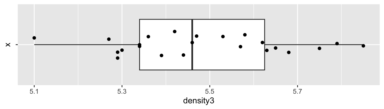

The data appears plausibly to be from a normal distribution, and there are no apparent outliers. Since the data was collected sequentially over time, we may wonder whether there is any time dependence. A full examination of that is beyond the scope of this text, but we can examine a scatterplot of the values against observation number to see if there are any obvious patterns. We would also want to confirm with the experimenter that the observation order given in the data set is the order in which the observations were made.

cavendish %>%
  mutate(observation = 1:29) %>%
  ggplot(aes(x = observation, y = density3)) +
  geom_point()

There is no obvious pattern to the data, so we assume independence.

t.test(cavendish$density3, mu = 5.5155)

## 
##  One Sample t-test
## 
## data:  cavendish$density3
## t = -0.80648, df = 22, p-value = 0.4286
## alternative hypothesis: true mean is not equal to 5.5155
## 95 percent confidence interval:
##  5.401134 5.565822
## sample estimates:
## mean of x 
##  5.483478

We get a 95% confidence interval of \((5.40, 5.57)\), which does contain the current accepted value of 5.5155. We also obtain a \(p\)-value of .4286, so we would not reject \(H_0: \mu = 5.5155\) at the \(\alpha = .05\) level. We conclude that there is not sufficient evidence that the mean value of Cavendish’s experiment differed from the currently accepted value.

8.4 One-sided confidence intervals and hypothesis tests

In this short section, we introduce one-sided confidence intervals and hypothesis tests through an example.

Consider the cows_small data set from the fosdata package. If you are interested in the full, much more complicated data set, that can be found in fosdata::cows.

cows_small <- fosdata::cows_small

On hot summer days, cows in Davis, CA were sprayed with water for three minutes, and the change in temperature as measured at the shoulder was measured.⁵⁶ There are three different treatments of cows, including the control, which we ignore in this example. For now, we are only interested in the nozzle type tk_0_75. In this case, we have reason to believe before the experiment begins that spraying the cows with water will lower their temperature. So, we are not as much interested in detecting a change in temperature, as a decrease in temperature. Additionally, should it turn out by some oddity that spraying the cows with water increased their temperature, we would not recommend spraying cows with water in order to increase their temperature. We will only make a recommendation of using nozzle tk_0_75 if it decreases the temperature of the cows. This changes our analysis.

Alert 8.4

The same data cannot be used to decide whether to do a one-sided test and for the test itself. Doing so will inflate the \(p\)-value by a factor of 2 and is highly inappropriate.

Before proceeding, let’s look at a plot of the data.

ggplot(cows_small, aes(x = "", y = tk_0_75)) +
  geom_boxplot(outlier.size = -1) +
  geom_jitter(height = 0, width = 0.2) +
  coord_flip()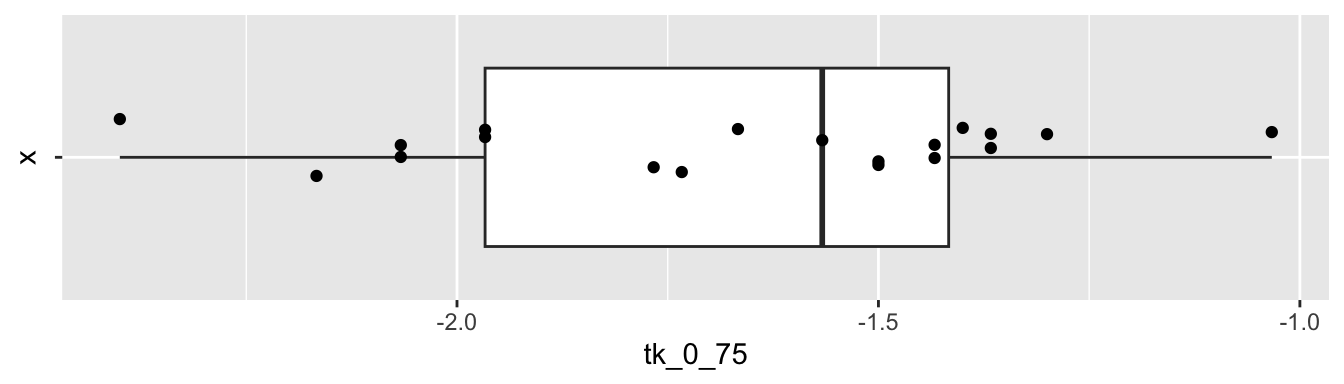

The data seems to plausibly come from a normal distribution, there don’t seem to be any outliers, and we assume that the observations are independent.

Let \(\mu\) denote the true (unknown) mean change in temperature as measured at the shoulder of cows sprayed with the tk_0_75 nozzle for three minutes. We will construct a 98% confidence interval for \(\mu\) of the form \((-\infty, u)\). If \(u = -1\) for example, this would mean that we are 98% confident that the drop in temperature is at least one degree Celsius.

We will also perform the following hypothesis test:

• \(H_0: \mu \ge 0\) vs.

• \(H_a: \mu < 0\)

If we reject \(H_0\) in favor of \(H_a\), then we are concluding that the temperature of cows sprayed with tk_0_75 will drop on average.

The outcomes that are most likely under \(H_a\) relative to \(H_0\) are of the form \(\overline{X} < u\), so the rejection region for this test is \[ \frac{\overline{X} - \mu_0}{S/\sqrt{n}} < t_{.98} \] where \(t_{.98}\) = qt(.98, 18, lower.tail = FALSE) = -2.213703. After collecting the data, we will reject the null hypothesis if \(t = \frac{\overline{x} - 0}{s/\sqrt{n}} < -2.213703\), and the \(p\)-value is pt(t, 18).

R computes this for us using t.test with alternative = "less":

t.test(cows_small$tk_0_75, mu = 0, alternative = "less", conf.level = .98)

## 
##  One Sample t-test
## 
## data:  cows_small$tk_0_75
## t = -20.509, df = 18, p-value = 3.119e-14
## alternative hypothesis: true mean is less than 0
## 98 percent confidence interval:
##       -Inf -1.488337
## sample estimates:
## mean of x 
## -1.668421

Note that the \(p\)-value is given as we discussed above via:

pt(-20.509, 18)

## [1] 3.119495e-14

The \(p\)-value associated with the hypothesis test is \(p = 3.1 \times 10^{-14}\), so we would reject \(H_0\) that the mean temperature change is zero. We conclude that use of nozzle TK-0.75 is associated with a mean drop in temperature after three minutes as measured at the shoulder of the cows.

The confidence interval for the change in temperature associated with nozzle TK-0.75 is read from the output of t.test as \((-\infty, -1.49)\) degrees Celsius. That is, we are 98% confident that the mean drop in temperature is at least 1.49 degrees Celsius.

8.5 Assessing robustness via simulation

In the chapter up to this point, we have assumed that the underlying data is a random sample from a normal distribution. Let’s look at how various types of departures from those assumptions affect the validity of our statistical procedures. For the purposes of this discussion, we will restrict to hypothesis testing at a specified \(\alpha\) level, but our results will hold for confidence intervals and reporting \(p\)-values just as well.

Our point of view is that if we design our hypothesis test at the \(\alpha = 0.1\) level, say, then we want to incorrectly reject the null hypothesis 10% of the time. That is how our test is designed. In order to talk about this, we introduce some new terminology.

Definition 8.13

For a hypothesis test, a type I error is rejecting the null hypothesis when it is true. The effective type I error rate of a hypothesis test is the probability that a type I error will occur.

When all of the assumptions of a hypothesis test at the \(\alpha\) level are met, the effective type I error rate is exactly \(\alpha\). If one or more of the assumptions are violated, then we want to estimate the effective type I error rate and compare it to \(\alpha\). If the effective error rate is far from \(\alpha\), then the test is not performing as designed. We will note whether the test makes too many type I errors or too few, but the main objective is to see whether the test is performing as designed.

Our first observation is that when the sample size is large, then the Central Limit Theorem tells us that \(\overline{X}\) is approximately normal. Since the test statistic \(T\) is also approximately normal when \(n\) is large, this gives us some measure of protection against departures from normality in the underlying population.

In the sequel, it will be very useful to pull out the \(p\)-value of the t.test. Let’s see how we can do that. We begin by doing a t.test on “garbage data” just to see what t.test returns.

str(t.test(c(1, 2, 3)))

## List of 10
##  $ statistic  : Named num 3.46
##   ..- attr(*, "names")= chr "t"
##  $ parameter  : Named num 2
##   ..- attr(*, "names")= chr "df"
##  $ p.value    : num 0.0742
##  $ conf.int   : num [1:2] -0.484 4.484
##   ..- attr(*, "conf.level")= num 0.95
##  $ estimate   : Named num 2
##   ..- attr(*, "names")= chr "mean of x"
##  $ null.value : Named num 0
##   ..- attr(*, "names")= chr "mean"
##  $ stderr     : num 0.577
##  $ alternative: chr "two.sided"
##  $ method     : chr "One Sample t-test"
##  $ data.name  : chr "c(1, 2, 3)"
##  - attr(*, "class")= chr "htest"

It’s a list of 10 things, and we can pull out the \(p\)-value by using t.test(c(1,2,3))$p.value.

8.5.1 Symmetric, light tails

As a model for a symmetric, light-tailed population, we choose a uniform random variable.

Example 8.14

Estimate the effective type I error rate in a \(t\)-test of \(H_0: \mu = 0\) versus \(H_a: \mu\not = 0\) when the underlying population is uniform on the interval \((-1,1)\). Take a sample size of \(n = 10\) and test at the \(\alpha = 0.1\) level.

In this scenario, \(H_0\) is true. So, we are going to estimate the probability of rejecting \(H_0\). Let’s build up our replicate function step by step.

runif(10, -1, 1) # Sample of size 10 from uniform rv

##  [1] -0.4689827 -0.2557522  0.1457067  0.8164156 -0.5966361  0.7967794
##  [7]  0.8893505  0.3215956  0.2582281 -0.8764275

t.test(runif(10, -1, 1))$p.value # p-value of test

## [1] 0.5089686

t.test(runif(10, -1, 1))$p.value < .1 # true if we reject

## [1] FALSE

mean(replicate(10000, t.test(runif(10, -1, 1))$p.value < .1))

## [1] 0.1007

Our result is 10.07%. That is really close to 10%, which is what the test is designed to give. The \(t\)-test is working well in this situation.

Remark

How do we know we have run enough replications to get a reasonable estimate for the probability of a type I error? Well, we don’t. So we repeat our experiment a couple of times:

mean(replicate(10000, t.test(runif(10, -1, 1))$p.value < .1))

## [1] 0.0968

mean(replicate(10000, t.test(runif(10, -1, 1))$p.value < .1))

## [1] 0.0993

The results are pretty similar each time. That’s reason enough to believe the true type I error rate is relatively close to what we computed.

Tryit 8.4

Estimate the effective type I error rate as in Example 8.14 for \(\alpha = .05\) and \(\alpha = .01\), and for \(n = 10\) and \(n = 20\). How close are the effective error rates to the designed values?

8.5.2 Skew

As a model for a skewed population, we use an exponential random variable.

Example 8.15

Estimate the effective type I error rate in a \(t\)-test of \(H_0: \mu = 1\) versus \(H_a: \mu\not = 1\) when the underlying population is exponential with rate 1. Use a sample of size \(n = 20\) and test at the \(\alpha = 0.05\) level.

We have to specify the null hypothesis mu = 1 in the \(t\)-test so that \(H_0\) will be true.

mean(replicate(10000, t.test(rexp(20, 1), mu = 1)$p.value < .05))

## [1] 0.0824

Here we get an effective type I error rate (rejecting \(H_0\) when \(H_0\) is true) of 8.24%. Since the test is designed to have a 5% error rate, we made 1.648 times as many type I errors as we should have. Most people would argue that the test is not working as designed.

Tryit 8.5

Repeat Example 8.15 with sample size of \(n=50\) for \(\alpha = .1\), \(\alpha = .01\) and \(\alpha = .001\). We recommend increasing the number of replications as \(\alpha\) gets smaller. Don’t go overboard though, because this can take a while to run.

You should see that at \(n = 50\), the effective type I error rate gets worse in relative terms as \(\alpha\) gets smaller. The estimate at the \(\alpha = .001\) level is an effective error rate more than 6 times what is designed! That is unfortunate, because small \(\alpha\) are exactly what we are interested in. That’s not to say that \(t\)-tests are useless in this context, but \(p\)-values should be interpreted with some level of caution when the underlying population is skewed. In particular, it would be misleading to report a \(p\)-value with 7 significant digits, as R does by default.

We simulate the effective type I error rates for \(H_0: \mu = 1\) versus \(H_a: \mu \not= 1\) at \(\alpha = .1, .05, .01\) and \(.001\) levels for sample sizes \(N = 10, 20, 50, 100\) and 200.

effectiveError <- sapply(c(.1, .05, .01, .001), function(y) {
  sapply(c(10, 20, 50, 100, 200), function(x) {
    mean(replicate(20000, t.test(rexp(x, 1), mu = 1)$p.value < y))
  })
})
colnames(effectiveError) <- c(".1", ".05", ".01", ".001")
rownames(effectiveError) <- c("10", "20", "50", "100", "200")
effectiveError

##         0.1    0.05    0.01   0.001
## 10  0.14310 0.10015 0.04600 0.01460
## 20  0.12730 0.08085 0.03240 0.01120
## 50  0.11475 0.06850 0.02310 0.00605
## 100 0.10945 0.05800 0.01755 0.00365
## 200 0.10135 0.05345 0.01490 0.00235

Figure 8.4 plots these results, illustrating how the test improves as sample size increases.

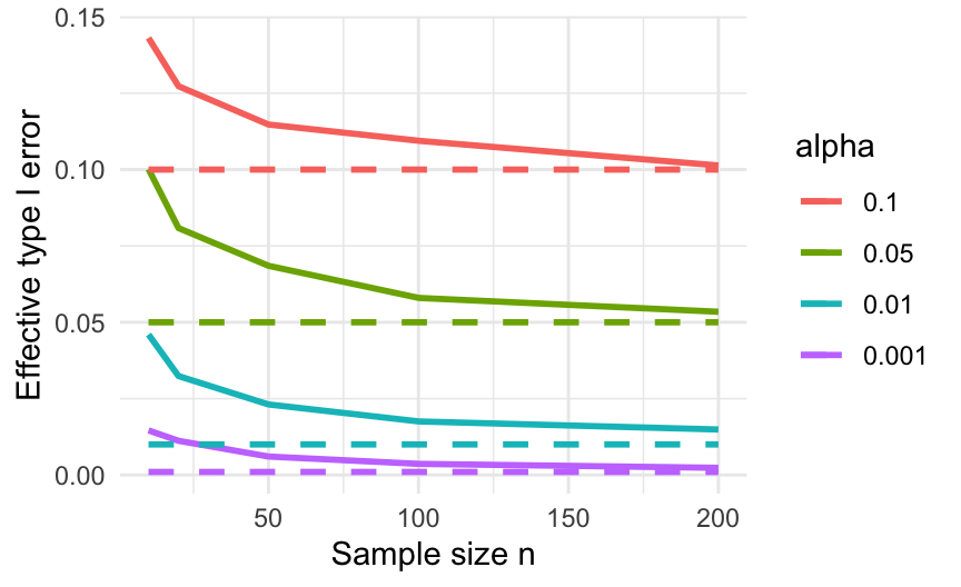
Figure 8.4: Effective type I errors when applying a \(t\)-test to exponential data. Dashed lines show the type I error a correctly behaving test should have.

8.5.3 Heavy tails and outliers

If the results of the preceding section didn’t convince you that you need to understand your underlying population before applying a \(t\)-test, then this section will. A typical “heavy tail” distribution is the \(t\) random variable. Indeed, the \(t\) random variable with 1 or 2 degrees of freedom doesn’t even have a finite standard deviation!

Example 8.16

Estimate the effective type I error rate in a \(t\)-test of \(H_0: \mu = 0\) versus \(H_a: \mu\not = 0\) when the underlying population is \(t\) with 3 degrees of freedom. Take a sample of size \(n = 30\) and test at the \(\alpha = 0.1\) level.

mean(replicate(20000, t.test(rt(30, 3), mu = 0)$p.value < .1))

## [1] 0.09535

Not too bad. It seems that the \(t\)-test has an effective error rate less than how the test was designed.

Example 8.17

Let’s model data that contains an outlier. Assume a population is normal with mean 3 and standard deviation 1. However, there is an error in measurement, and one of the values is multiplied by 100 due to a missing decimal point. Estimate the effective type I error rate in a \(t\)-test of \(H_0: \mu = 3\) versus \(H_a: \mu\not = 3\) at the \(\alpha = 0.1\) level with sample size \(n = 100\).

mean(replicate(10000, {
  dat <- rnorm(100, 3, 1)
  dat[1] <- dat[1] * 100
  t.test(dat, mu = 3)$p.value < .1
}))

## [1] 2e-04

The mean is \(0.0002\) which means that the test only rejected the null hypothesis 2 of the 10,000 times we ran it. This is terrible, because the test is designed to reject \(H_0\) 1,000 times out of 10,000!

Both examples in this section resulted in fewer type I errors than expected. That may seem like a good thing. However, one way to avoid type I errors is to simply never reject \(H_0\), and that’s what is happening here. Using a \(t\)-test on heavy-tailed data or data with outliers results in a test with very low power, a concept we will explore with one example here and in greater detail in Section 8.7.

Example 8.18

Use the same population as in Example 8.17, a normal population with mean 3 and standard deviation 1, with an outlier caused by multiplying one of the values by 100. Change the null hypothesis to \(H_0: \mu = 7\), so it is no longer true.

Estimate the percentage of time you would correctly reject \(H_0\) at the \(\alpha = 0.1\) level with sample size \(n = 100\).

We have a null hypothesis for \(\mu\) that is 4 standard deviations away from the true value of \(\mu\). That should be easy to spot. Let’s see.

mean(replicate(20000, {
  dat <- c(rnorm(99, 3, 1), 100 * rnorm(1, 3, 1))
  t.test(dat, mu = 7)$p.value < .1
}))

## [1] 0.0706

We have estimated the probability of correctly rejecting the null hypothesis as 0.0706. The value 0.0706 is the power of the test. There is no “right” value for the power, but 0.0706 is very low. We only detect a difference of four standard deviations (which is huge!) about 7% of the time that we run the test. The test is hardly worth doing.

8.5.4 Independence

The \(t\)-test assumes that data values are independent of each other. What happens when that assumption is violated? We investigate via simulation, looking at two different types of dependence that frequently occur in real experiments. One is when the sample consists of repeated measures on a common observational unit, and the other is when there is dependence between observations when ordered by another variable such as time.

Example 8.19

Suppose that an experimental design consists of multiple measurements from a single unit. For example, we might measure the temperature of 20 people five times each in order to determine the mean temperature of healthy adults. In this case, it would be a mistake to assume that the observations are independent.

Assume that the true mean temperature of healthy adults is 98.6 with a standard deviation of 0.7. We model repeated samples as follows. First, choose a mean temperature for each of the 20 people. Then, assume that each person’s own temperatures are centered at their personal mean temperature with standard deviation 0.5.

# choose a mean temperature for each person
people_means <- rnorm(20, 98.6, .7)
# take five readings of each person
temps <- rnorm(100, mean = rep(people_means, 5), sd = 0.5)
head(temps)

## [1]  98.65737 100.25115  98.23785  97.59733  97.89514  98.82903

We now test \(H_0 : \mu = 98.6\) using all 100 data points, and then replicate this test to estimate the type I error rate:

sim_data <- replicate(1000, {
  people_means <- rnorm(20, 98.6, .7)
  temps <- rnorm(100, mean = rep(people_means, 5), sd = 0.5)
  t.test(temps, mu = 98.6)$p.value
})
mean(sim_data < .05)

## [1] 0.344

The effective type I error rate in this case is much larger than 5%! This is strong evidence that one should not ignore this type of dependence in data.

Tryit 8.6

1. Change the population standard deviation from 0.7 to 2. Does the effective type I error rate increase or decrease?
2. Change the personal standard deviation from 0.5 to 2 (while returning the population standard deviation to 0.7). Does the effective type I error rate increase or decrease?
3. Return the standard deviations to 0.7 and 0.5, and now take 10 readings from 10 different people. What happens to the effective type I error rate?

Example 8.20

This example explores dependence between observations when ordered by a second variable. A common special case is when the observations are ordered via time. For example, if you wish to determine whether the high temperatures in a specific city in 2020 are higher than they were in 2000, you could subtract the high temperatures in 2000 from those in 2020. The resulting data would likely be dependent on time: if it were warmer in 2020 on February 1, then it will usually be warmer in 2020 on February 2.

In order to simulate this, we will create 100 data points \(x_1, \ldots, x_{100}\) such that \(x_1\) is standard normal, and \(x_n = 0.5 x_{n - 1} + z_n\), where \(z_n\) is again standard normal. We see that the \(n^\text{th}\) data point will depend on the previous data point relatively strongly, and on ones before that to a smaller extent.

We show two ways to simulate data of this type. The first uses a while loop, which we only covered briefly in the Loops in R vignette at the end of Chapter 3. Readers who do not wish to see this can safely bypass to the built-in R function which samples from this distribution.

x <- rep(NA, 100) # create a vector of length 100 that we will fill in below
x[1] <- rnorm(1)
i <- 2
while (i < 101) {
  x[i] <- .5 * x[i - 1] + rnorm(1)
  i <- i + 1
}
plot(x, type = "l")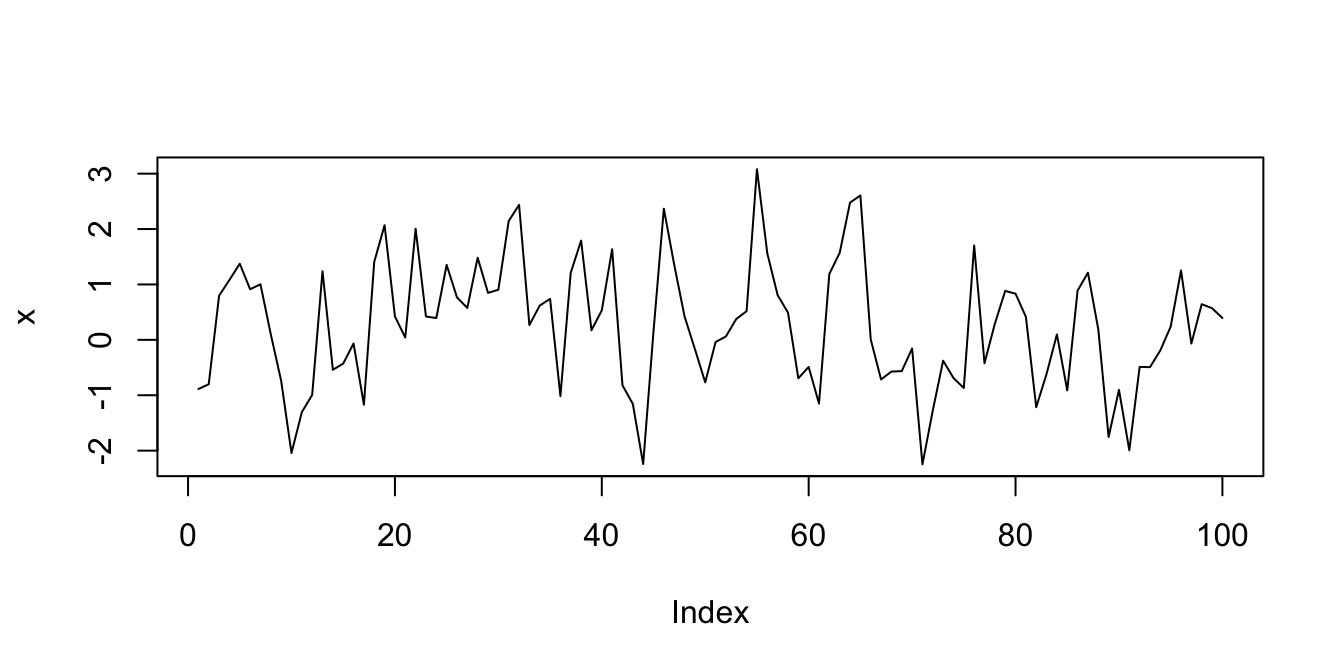

This is a common enough process that there is a built-in R function arima.sim which does essentially this and much, much more. For our purposes, we only care about the ar parameter in the model list. That is the value \(c\) such that \(x_n = c x_{n - 1} + z_n\).

x <- arima.sim(model = list(ar = .5), n = 100)

Now we suppose that we have data of this type, and we estimate the effective type I error rate when testing \(H_0: \mu = 0\) versus \(H_a: \mu \not= 0\).

sim_data <- replicate(10000, {
  x <- arima.sim(model = list(ar = .5), n = 100)
  t.test(x, mu = 0)$p.value
})
mean(sim_data < .05)

## [1] 0.2619

The effective type I error rate is much higher than the desired rate of \(\alpha = .05\). It would be inappropriate to use a one sample \(t\)-test on data of this type.

Tryit 8.7

Change the ar parameter to .1 and to .9 and estimate the effective type I error rate. Which one is performing closest to the desired rate of \(\alpha = .05\)?

8.5.5 Summary

When doing \(t\)-tests on populations that are not normal, the following types of departures from design were noted:

1. When the underlying distribution is skewed, the exact \(p\)-values should not be reported to many significant digits (especially the smaller they get). If a \(p\)-value close to the \(\alpha\) level of a test is obtained, then we would want to note the fact that we are unsure of our \(p\)-values due to skewness, and fail to reject.

2. When the underlying distribution has outliers, the power of the test is severely compromised. A single outlier of sufficient magnitude will force a \(t\)-test to never reject the null hypothesis. If your population has outliers, you do not want to use a \(t\)-test.

3. When the sample is not independent, then the source and type of dependence will need to be understood and adjusted for. It is not typically appropriate to use t.test without making these adjustments.

Alert 8.5

Boxplots created in base R and in ggplot2 show outliers in the data. Outliers that show up in boxplots are not necessarily problematic for t.test.

Tryit 8.8

Generate a sample of size 50 from a normal population, and plot it with a boxplot. Do you see outliers? Repeat this a few times to get a sense of how often apparent outliers show up in perfectly normal data.

For real experiments with apparent outliers, run simulations with normal data and compare. If the number and especially the magnitude of outliers in your data are worse than what you see in simulations, then you are right to be concerned.

8.6 Two sample hypothesis tests

This section presents hypothesis tests for comparing the means of two populations. In this situation, we have two populations that we are sampling from, and we ask whether the mean of population one differs from the mean of population two.

For tests of the mean, we must assume the underlying populations are normal, or that we have enough samples so that the Central Limit Theorem takes hold. We are also as always assuming that there are no outliers. Remember, outliers can kill \(t\)-tests. Both the one sample and the two sample variety.

For two sample tests, the (unknown) means of the two populations are \(\mu_1\) and \(\mu_2\). Our hypotheses are:

• \(H_0: \, \mu_1 = \mu_2\) versus
• \(H_a: \, \mu_1 \not= \mu_2\).

As with one sample tests, the alternate hypothesis may be one-sided if justified by the experiment. One-sided tests have \(H_a: \mu_1 \leq \mu_2\) or \(H_a: \mu_1 \geq \mu_2\). One-sided tests should be used judiciously, and the same warnings apply as were presented in Section 8.4.

The most straightforward experiment that results in two independent samples is a study comparing the same measurement on two different populations. In this case, a sample is chosen from population one, a second sample is chosen independently from population two, and both samples are measured. Another common setting is a controlled experiment. In a controlled experiment, the two populations are a group that receives some treatment and a control group that does not⁵⁷. Subjects are randomly assigned to either the control or treatment group. In both of these designs, the two independent samples \(t\)-test is appropriate.

The two sample paired \(t\)-test is used when data comes in pairs. Pairs may be two different subjects matched for some common traits, or they may come from two measurements on a single subject.

For example, suppose you wish to determine whether a new fertilizer increases the mean number of apples that apple trees produce. Here are three reasonable experimental designs:

Design 1

Randomly select two samples of trees. Apply fertilizer to one sample and leave the other sample alone as a control group. At the end of the growing season, count the apples on each tree in each group.

Design 2

Choose one sample of trees for the experiment. Count the number of apples on each tree after one growing season. The next season, apply the fertilizer and count the number of apples again.

Design 3

Carefully choose trees in pairs, so that each pair of trees is of similar maturity and will grow under similar conditions (soil quality, water, and sunlight). Randomly assign one tree of each pair to receive fertilizer and the other to act as control. Count the number of apples on the fertilized trees and the unfertilized trees.

Image credit: George Chernilevsky.Image Credit
George Chernilevsky. Public domain. https://commons.wikimedia.org/wiki/File:Apples_on_tree_2011_G1.jpg

In design 1, the two independent samples \(t\)-test is appropriate. Data from this experiment will likely be in long form, with a two-valued grouping variable in one column and a measurement variable giving apple counts in a second column.

Designs 2 and 3 result in paired data. The measures in the two populations are dependent. You expect there to be some relationship between the number of apples you count on each pair. For example, big trees would have more apples each season than small trees. In general, it is a hard problem to deal with dependent data, but paired data is a dependency we can handle with the two sample paired \(t\)-test.

In designs 2 and 3, the data will likely be in wide form for analysis: each row representing a pair, and two columns with apple counts. In design 2, the rows are individual trees and the columns are the two measurements, before and after. In design 3, the rows are pairs of trees and the columns are measurements for the fertilized and unfertilized member of each pair. Table 8.2 shows the typical structure of data for each of these designs.

Table 8.2: Data from three experimental designs: independent samples, before/after, and matched pairs.

group apples fertilized 660 control 533 fertilized 418 fertilized 549 control 574 fertilized 558

before after 469 496 651 498 539 594 438 582 279 559 612 592

fertilized control 578 353 507 452 301 542 562 636 494 490 484 539

8.6.1 Two independent samples \(t\)-test

For the two independent samples \(t\)-test, we require data \(x_{1,1},\dotsc,x_{1,n_1}\) drawn from one population and \(x_{2,1},\dotsc,x_{2,n_2}\) drawn independently from a second population.

Assumptions 8.2

• The samples are independent.
• The underlying populations are normal, or the sample sizes are large.
• There are no outliers.

We calculate the means of the two samples \(\overline{x}_1\) and \(\overline{x}_2\) and their variances \(s_1^2\) and \(s_2^2\). The test statistic is given by

\[ t = \frac{\overline{x}_1 - \overline{x}_2}{\sqrt{s_1^2/n_1 + s_2^2/n_2}}. \]

If the assumptions are met, then the test statistic has a \(t\) distribution with a complicated (and non-integer) df. In the past, when computations like this were made by hand, it was common to add an assumption of “equal variances” and use both populations to estimate the variance, in which case the expression for \(t\) simplifies somewhat. In general, it is a more conservative approach not to assume the variances of the two populations are equal, and we generally recommend not to assume equal variance unless you have a good reason for doing so.

In R, the two independent samples \(t\)-test is performed with the syntax t.test(value ~ group, data = dataset). Here value is the name of the measurement variable, group should be a variable that takes on exactly two values, and dataset is the name of the data set. The value ~ group expression is known as a formula, and should be read as “value which depends on group.” The ~ is a tilde character. We will see this syntax used frequently in Chapter 11 when performing regression analysis.

Example 8.21

We return to the brake data in the fosdata package. Recall that we were interested in whether there is a difference in the mean time for an older person and the mean time for a younger person to release the brake pedal after it unexpectedly causes the car to speed up.

Let \(\mu_1\) be the mean time to release the pedal for the older group, and let \(\mu_2\) denote the mean time of the younger group in milliseconds.

\[ H_0: \mu_1 = \mu_2 \] versus \[ H_a: \mu_1\not= \mu_2 \]

It might be reasonable to do a one-sided test here if you have data or other evidence suggesting that older drivers are going to have slower reaction times, but we will stick with the two-sided tests.

Let’s think about the data that we have for a minute. Do we expect the reaction times to be approximately normal? How many samples do we have? We compute the mean, sd, skewness, and number of observations in each group and also plot the data.

brake <- fosdata::brake
brake %>%
  group_by(age_group) %>%
  summarize(
    mean = mean(latency_p2),
    sd = sd(latency_p2),
    skew = e1071::skewness(latency_p2),
    N = n()
  )

## # A tibble: 2 × 5
##   age_group  mean    sd  skew     N
##   <chr>     <dbl> <dbl> <dbl> <int>
## 1 Old        956. 242.  1.89     40
## 2 Young      664.  95.9 0.780    40

ggplot(brake, aes(x = age_group, y = latency_p2)) +
  geom_boxplot(outlier.size = -1) +
  geom_jitter(height = 0, width = .2)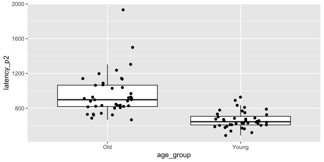

The older group in particular is right skewed, and there is one extreme⁵⁸ outlier among the older drivers. These are concerns, but with 80 observations our assumptions are met well enough. We tell t.test to break up latency_p2 by age_group and perform a two sample \(t\)-test.

t.test(latency_p2 ~ age_group, data = brake)

## 
##  Welch Two Sample t-test
## 
## data:  latency_p2 by age_group
## t = 7.0845, df = 50.97, p-value = 4.014e-09
## alternative hypothesis: true difference in means between group Old and group Young is not equal to 0
## 95 percent confidence interval:
##  208.7430 373.8345
## sample estimates:
##   mean in group Old mean in group Young 
##            955.7747            664.4859

We reject the null hypothesis that the two means are the same (\(p = 4.0 \times 10^{-9}\)). A 95% confidence interval for the difference in mean times is \((209, 374)\) ms. That is, we are 95% confident that the mean time for older drivers is between 209 and 374 ms slower than the mean time for younger drivers.

In Exercise 8.40, you are asked to redo this analysis after removing the largest older driver outlier. When doing so, you will see that the skewness is improved, the \(p\)-value gets smaller, and the confidence interval gets more narrow. Therefore, we have no reason to doubt the validity of the work we did with the outlier included.

Tryit 8.9

Is there a significant difference between young and old drivers in the mean time to press the brake after seeing the red light (latency_p1)?

8.6.2 Paired two sample \(t\)-test

For the paired two sample \(t\)-test, we require data \(x_{1,1},\dotsc,x_{1,n}\) drawn from one population and \(x_{2,1},\dotsc,x_{2,n}\) drawn from a second population. The data come in pairs, so that \(x_{1,i}\) and \(x_{2,i}\) are not independent.

Assumptions 8.3

• The samples are paired.
• The underlying populations are normal, or the sample size is large.
• There are no outliers.

If we compute the difference \(d_i = x_{1,i} - x_{2,i}\) for each pair, then the resulting differences will be independent and contain information about which population is larger. Then we simply perform a one sample \(t\)-test to test the differences against zero. The mean and variance of \(d\) are \(\overline{d} = \overline{x}_1 - \overline{x}_2\) and \(s_d^2\). So the test statistic is

\[ T = \frac{\overline{x}_1 - \overline{x}_2}{s_d/\sqrt{n}}. \]

When the test assumptions are met, \(T\) will have the \(t\) distribution with \(n-1\) degrees of freedom.

In R, the syntax for a paired \(t\)-test is t.test(dataset$var1, dataset$var2, paired = TRUE).

Alert 8.6

It is possible to perform a paired \(t\)-test on long format data with formula notation value ~ group. This requires you to be sure that the data pairs are in order. More often than not, long format data is unpaired, and using formula notation to perform a paired test is a mistake.

Example 8.22

Return to the cows_small data set in the fosdata package. We wish to determine whether there is a difference between nozzle TK-0.75 and nozzle TK-12 in terms of the mean amount that they cool down cows in a three-minute period.

Let \(\mu_1\) denote the mean change in temperature of cows sprayed with TK-0.75 and let \(\mu_2\) denote the mean change in temperature of cows sprayed with TK-12. Our null hypothesis is \(H_0: \mu_1 = \mu_2\) and our alternative is \(H_a: \mu_1\not= \mu_2\). According to the manufacturer of the TK-0.75, it sprays 0.4 liters per minute at 40 PSI, while the TK-12 sprays 4.5 liters per minute. Since the TK-12 sprays considerably more water, it would be worth considering a one-sided test in this case. However, we don’t know any other characteristics of the nozzles which might mitigate the flow advantage of the TK-12, so we stick with a two-sided test.

The data is in wide format, with one column for each nozzle type. To check assumptions, we compute and plot the difference variable. Here we chose to use a qq plot but a histogram or boxplot would have also been appropriate.

cows_small <- fosdata::cows_small
ggplot(cows_small, aes(sample = tk_0_75 - tk_12)) +
  geom_qq() +
  geom_qq_line()

The distribution is somewhat heavy-tailed but good enough to proceed. We perform the paired two sample \(t\)-test.

t.test(cows_small$tk_12, cows_small$tk_0_75, paired = TRUE)

## 
##  Paired t-test
## 
## data:  cows_small$tk_12 and cows_small$tk_0_75
## t = -1.5118, df = 18, p-value = 0.1479
## alternative hypothesis: true mean difference is not equal to 0
## 95 percent confidence interval:
##  -0.31023781  0.05058868
## sample estimates:
## mean difference 
##      -0.1298246

We find a 95% confidence interval for the difference in the means to be \((-0.31, 0.05)\), and we do not reject \(H_0\) at the \(\alpha = .05\) level (\(p\) = .1479). We cannot conclude that there is a difference in the mean temperature change associated with the two nozzles.

Tryit 8.10

Is there a significant difference in the mean temperature change between the TK-0.75 nozzle and the control?

8.7 Type II errors and power

Up to this point, we have been concerned about the probability of incorrectly rejecting the null hypothesis when the null hypothesis is true. There is another type of error that can occur, however, and that is failing to reject the null hypothesis when the null hypothesis is false.

Definition 8.23

In a hypothesis test,

• A type I error is rejecting the null when it is true.
• A type II error is failing to reject the null when it is false.

Definition 8.24

The power of a test is defined to be one minus the probability of a type II error. That is, power is the probability of correctly rejecting the null hypothesis.

One issue that arises is that the null hypothesis is (usually) a simple hypothesis; that is, it consists of a complete specification of parameters, while the alternative hypothesis is often a composite hypothesis; that is, it consists of parameters in a range of values. Therefore, when we say the null hypothesis is false, we are not completely specifying the distribution of the population. For this reason, the type II error is a function that depends on the value of the parameter(s) in the alternative hypothesis.

The examples in this section imagine we are designing an experiment to collect data like fosdata::normtemp, which measured body temperature and heart rate of 130 healthy adults.

Example 8.25

Suppose we wish to conduct an experiment to determine if the mean heart rate of healthy adults is 80 beats per minute. Let \(\mu\) be the population mean heart rate. Then the hypotheses are:

• \(H_0: \mu = 80.\)
• \(H_a: \mu \neq 80.\)

With a sample size of \(n=130\) and significance level \(\alpha = 0.01\), what is the probability of a type II error?

Our plan is to simulate the experiment. However, for a type II error to happen, the alternate hypothesis must be true. The alternate hypothesis does not tell us the population distribution, so we must make assumptions about it.

We start by assuming the population heart rate is normally distributed. This is reasonable, as many physiological measurements are normal.

Next, assume the true population mean is 78. Of course, there is no point in performing the experiment if we know that \(\mu = 78\), but the hypothetical computation will still be useful. It will tell us the probability we fail to detect a difference of 2 bpm with our experimental setup, or equivalently the power our test will have to detect such a difference.

Finally, we need the population standard deviation. The American Heart Association says that 60-100 bpm is a range for normal heart rate. We interpret to mean that about 99% of healthy adult heart rates will fall in this range, so we will estimate the standard deviation to be (100 - 60)/6 = 6.67 bpm.⁵⁹

Now that the alternate hypothesis is specified, we can perform a simulation. Start by taking a sample of size 130 from a normal distribution with mean 78 and standard deviation 6.67. Then compute the \(t\) statistic and determine whether \(H_0\) is rejected at the \(\alpha = 0.01\) level.

dat <- rnorm(130, 78, 6.67)
t_stat <- (mean(dat) - 80) / (sd(dat) / sqrt(130))
t_stat

## [1] -3.843193

qt(.005, 129) # critical value

## [1] -2.614479

Since t_stat is less than qt(.005, 129) we would (correctly) reject the null hypothesis. It is even easier to use the built-in R function t.test:

dat <- rnorm(130, 78, 6.67)
t.test(dat, mu = 80)$p.value > .01

## [1] FALSE

Next, repeatedly sample and then compute the percentage of times that the \(p\)-value of the test is greater than .01. That will be our estimate for the probability of a type II error.

simdata <- replicate(10000, {
  dat <- rnorm(130, 78, 6.67)
  t.test(dat, mu = 80)$p.value > .01
})
mean(simdata)

## [1] 0.2136

We get about a 0.2136 chance for a type II error in this case, or a power of 0.7864.

This experimental setup will be able to detect a 2 bpm difference in heart rate about 78.6% of the time.

For many experimental designs, simulation is the best way to compute power. However, the \(t\)-test on a normal population is simple enough mathematically that power computations are possible to do exactly. The built-in function power.t.test does this. It has the following arguments:

n

the number of samples

delta

the difference between the null and alternative mean

sd

the standard deviation of the population

sig.level

the \(\alpha\) significance level of the test

power

one minus the probability of a type II error

type

either one.sample, two.sample or paired, default is two

alternative

two.sided or one.sided, default is two

To use power.t.test, specify any four of the first five parameters. The function then solves for the unspecified parameter.

Example 8.26

With the experimental setup of Example 8.25, compute the power exactly.

The assumptions made in Example 8.25 for the simulation are exactly the inputs needed for power.t.test. The value of delta is 2, which is the difference between our null hypothesis \(\mu = 80\) and our assumed reality of \(\mu = 78\).

power.t.test(
  n = 130, delta = 2, sd = 6.67,
  sig.level = .01, type = "one"
)

## 
##      One-sample t test power calculation 
## 
##               n = 130
##           delta = 2
##              sd = 6.67
##       sig.level = 0.01
##           power = 0.7878322
##     alternative = two.sided

The power is 0.7878322, so the probability of a type II error is one minus that, or

1 - .7878322

## [1] 0.2121678

which is close to what we computed in the simulation.

A traditional approach in designing experiments is to specify the significance level and power, and use a simulation or power.t.test to determine what sample size is necessary to achieve that power. In order to do so, we must estimate the standard deviation of the underlying population and we must specify the effect size that we are interested in.

Sometimes prior work or a pilot study could be used to determine a reasonable effect size. Other times, we can pick a size that would be clinically significant (as opposed to statistically significant). Think about it like this: if the true mean body temperature of healthy adults is 98.59, would that make a difference in treatment or diagnosis? No. What about if it were 100? Then yes, that would make a difference in diagnoses! It is subjective and can be challenging to specify what delta to provide, but we should provide one that would make an important difference in some context.

Example 8.27

How large a sample is needed to detect a clinically significant difference in body temperature from 98.6 degrees with a power of 0.8?

The null hypothesis is that the mean temperature of healthy adults is 98.6 degrees. We estimate the standard deviation of the underlying population to be 0.3 degrees. After consulting with our subject area expert, we decide that a clinically significant difference from 98.6 degrees would be 0.2 degrees. That is, if the true mean is 98.4 or 98.8, then we want to detect it with power 0.8. The sample size needed is

power.t.test(
  delta = 0.2, sd = .3,
  sig.level = .01, power = 0.8, type = "one.sample"
)

## 
##      One-sample t test power calculation 
## 
##               n = 29.64538
##           delta = 0.2
##              sd = 0.3
##       sig.level = 0.01
##           power = 0.8
##     alternative = two.sided

We would need to collect 30 observations in order to have an appropriately powered test.

8.7.1 Effect size

We used the term effect size in Section 8.7 without really saying what we mean. A common measure of the effect size is given by Cohen’s \(d\).

Definition 8.28

Cohen’s \(d\) is given by \[ d = \frac{\overline{x} - \mu_0}{s}, \] the difference between the sample mean and the mean from the null hypothesis, divided by the sample standard deviation.

The parametrization of power.t.test is redundant in the sense that the power of a test only relies on delta and sd through the effect size \(d\). As an example, we note that when delta = .1 and sd = .5 the effect size is 0.2, as it also is when delta = .3 and sd = 1.5. Both of these give the same power:

power.t.test(n = 30, delta = .3, sd = 1.5, sig.level = .05, type = "one")

## 
##      One-sample t test power calculation 
## 
##               n = 30
##           delta = 0.3
##              sd = 1.5
##       sig.level = 0.05
##           power = 0.1839206
##     alternative = two.sided

power.t.test(n = 30, delta = .1, sd = .5, sig.level = .05, type = "one")

## 
##      One-sample t test power calculation 
## 
##               n = 30
##           delta = 0.1
##              sd = 0.5
##       sig.level = 0.05
##           power = 0.1839206
##     alternative = two.sided

It is common to report the effect size, especially when there is statistical significance. Effect sizes are often reported along with adjectives such as “small,” “medium,” or “large.” These adjectives are domain dependent, and what is a very small effect in one discipline could be a very large effect in another.

You do not want your test to be underpowered for two reasons. First, you likely will not reject the null hypothesis in instances where you would like to be able to do so. Second, when effect sizes are estimated using underpowered tests, they tend to be overestimated. This leads to a reproducibility problem, because when people design further studies to corroborate your study, they are using an effect size that is too high. Let’s run some simulations to verify. We assume that we have an experiment with effect size \(d=0.2\).

power.t.test(
  delta = 0.2, sd = 1, sig.level = .05,
  power = 0.25, type = "one"
)

## 
##      One-sample t test power calculation 
## 
##               n = 43.24862
##           delta = 0.2
##              sd = 1
##       sig.level = 0.05
##           power = 0.25
##     alternative = two.sided

This says when \(d = 0.2\), we need a sample size of 43 for the power to be 0.25. Remember, power this low is not recommended! We use simulation to estimate the percentage of times that the null hypothesis is rejected. We assume we are testing \(H_0: \mu = 0\) versus \(H_a: \mu \not=0\).

simdata <- replicate(10000, {
  dat <- rnorm(43, 0.2, 1)
  t.test(dat, mu = 0)$p.value
})
mean(simdata < .05)

## [1] 0.2416

And we see that indeed, we get about 25%, which is what power.t.test predicted. Note that the true effect size is 0.2. The estimated effect size from tests which are significant is given by:

simdata <- replicate(10000, {
  dat <- rnorm(43, 0.2, 1)
  ifelse(t.test(dat, mu = 0)$p.value < .05,
    abs(mean(dat)) / sd(dat),
    NA
  )
})
mean(simdata, na.rm = TRUE)

## [1] 0.4066708

We see that the mean estimated effect size is double the actual effect size, so we have a biased estimate for effect size. If we have an appropriately powered test, then this bias is much less.

power.t.test(
  delta = 0.2, sd = 1, sig.level = .05,
  power = 0.8, type = "one"
)

## 
##      One-sample t test power calculation 
## 
##               n = 198.1513
##           delta = 0.2
##              sd = 1
##       sig.level = 0.05
##           power = 0.8
##     alternative = two.sided

simdata <- replicate(10000, {
  dat <- rnorm(199, 0.2, 1)
  ifelse(t.test(dat, mu = 0)$p.value < .05,
    abs(mean(dat)) / sd(dat),
    NA
  )
})
mean(simdata, na.rm = TRUE)

## [1] 0.2252131

With power 0.8, the estimated effect size is only a little over the true value of 0.2.

8.8 Resampling

Resampling is a modern technique for doing statistical analyses. Commonly used techniques include the bootstrap, permutation tests and cross validation. This section covers using the bootstrap and permutation tests to perform inference on the mean when sampling from one or two populations. Cross validation is covered in the context of linear regression in Section 11.7. For more information on these techniques, see Efron and Tibshirani.⁶⁰

8.8.1 Bootstrapping

The key fact we used for inference on the mean in this chapter is that \[ \frac{\overline{X} - \mu_0}{S/\sqrt{n}} \] is a \(t\) random variable with \(n - 1\) degrees of freedom when \(X_1, \ldots, X_n\) is a random sample from a normal population with mean \(\mu_0\).

Bootstrapping provides an alternative approach for performing inference on the mean, where we estimate the sampling distribution of \(\overline{X}\) directly from the random sample that we obtain as data. The idea is to repeatedly resample with replacement from the data that we obtained, and compute the value \(\overline{X}\) for each resample. The obtained sample is an estimate for the distribution of \(\overline{X}\). In this section, we will illustrate the basic ideas of the bootstrap through examples.

Example 8.29

Consider the brake data set in the fosdata package. We will construct the sampling distribution for \(\overline{X}\). Let’s start by plotting a histogram of the data.

brake_old <- fosdata::brake %>%
  filter(age_group == "Old")
ggplot(brake_old, aes(x = latency_p1)) +
  geom_histogram() +
  scale_x_continuous(limits = c(300, 1300))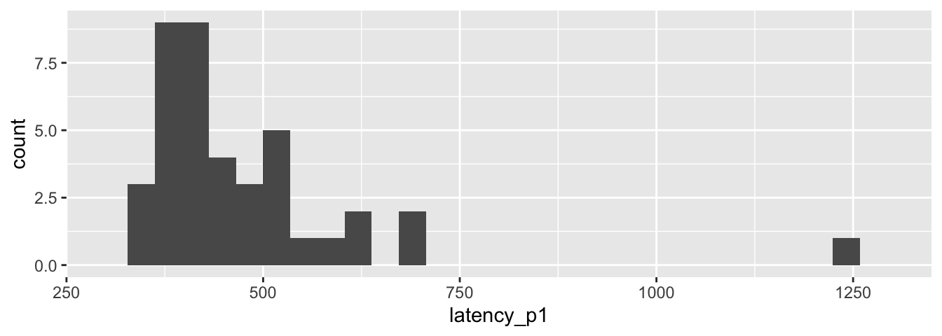

This latency data has mean 474.202 and does not appear to be normally distributed.

To bootstrap, we resample from the data with replacement. If we do this one time, here is what we get.

latency_p1_resample <- sample(brake_old$latency_p1, replace = TRUE)
data.frame(latency_p1_resample) %>% ggplot(aes(x = latency_p1_resample)) +
  geom_histogram() +
  scale_x_continuous(limits = c(300, 1300)) +
  geom_vline(xintercept = mean(latency_p1_resample), color = "red")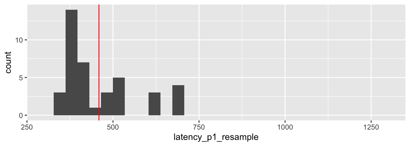

We see that the characteristics of this sample are similar to, but different from, the characteristics of the original data. In particular, the largest value in the original sample was not chosen in the bootstrap resample. If we repeat this, the largest value could be chosen once, twice or more times. The mean of the resample is 459.1, shown in red on the plot.

To estimate the sampling distribution of \(\overline{X}\), we resample many times and get many different possible values for the sample mean. Each sample mean represents one possible result of an experiment that was not run. Together, these resamples provide an estimate of the distribution of \(\overline{X}\). The histogram in Figure 8.5 is our estimate for the sampling distribution of \(\overline{X}\).

Xbar <- replicate(10000, {
  brake_lat <- sample(brake_old$latency_p1, replace = TRUE)
  mean(brake_lat)
})
data.frame(Xbar) %>% ggplot(aes(x = Xbar)) +
  geom_histogram()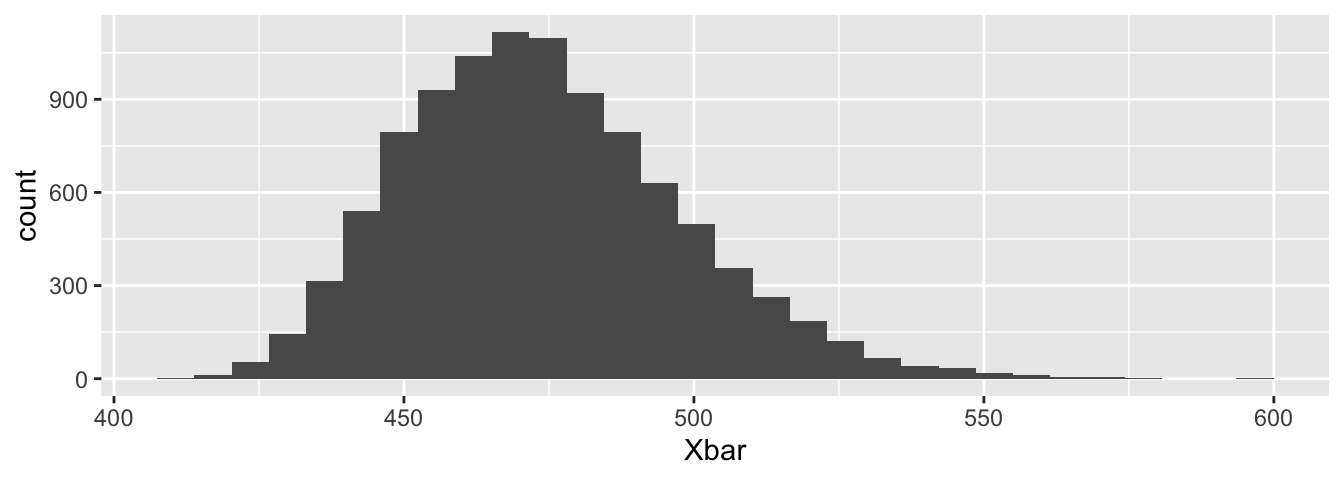

Figure 8.5: Bootstrap resampling estimate for the distribution of \(\overline{X}\).

Definition 8.30

Using bootstrapping, the \(100(1-\alpha)\%\) confidence interval is the interval from the \(\alpha/2\) to the \(1-\alpha/2\) quantiles of the bootstrap estimated sampling distribution.

The R function quantile computes quantiles of a numeric vector. Quantiles are often multiplied by 100 and referred to as percentiles, so that the 50th percentile is the 0.5 quantile and also the median of the data.

Example 8.31

Using the brake data, construct a 95% bootstrap confidence interval for \(\mu\), the mean latency in older drivers until they press the brake.

To compute the 95% confidence interval for the mean latency in older drivers, find the 0.025 and 0.975 quantiles of the \(\overline{X}\) distribution that was simulated in Example 8.29.

quantile(Xbar, c(.025, .975))

##     2.5%    97.5% 
## 434.0751 525.7794

The 95% confidence interval is 434 – 526. Compare this to the confidence interval computed using t.test:

t.test(brake_old$latency_p1)$conf.int

## [1] 425.4956 522.9084
## attr(,"conf.level")
## [1] 0.95

The bootstrap interval is narrower and both endpoints are higher, which one could attribute to the right skewness of this data.

The bootstrap method also works when we wish to create confidence intervals for other test statistics. For example, the trimmed mean removes a fraction of the most extreme values of a vector and then computes the mean. The trimmed mean is sometimes used in the presence of outliers, when we wish to understand the mean of the “typical” data from the population. The trimmed mean is implemented in R via mean with the argument trim, which is “the fraction (0 to 0.5) of observations to be trimmed from each end of [the vector] before the mean is computed.”

Example 8.32

Find a 95% bootstrap confidence interval for the mean after trimming by 10% on each side of the p1_latency for older drivers.

We first compute the trimmed mean. Note that this is the same as the mean after removing the smallest 4 and largest 4 values.

mean(brake_old$latency_p1, trim = 0.1)

## [1] 447.3073

mean(sort(brake_old$latency_p1)[-c(1:4, 37:40)])

## [1] 447.3073

We then follow the same procedure as above, sampling with replacement from the population and computing the trimmed mean each time.

Xbar_trimmed <- replicate(10000, {
  latency_p1_resample <- sample(brake_old$latency_p1, replace = TRUE)
  mean(latency_p1_resample, trim = 0.1)
})
quantile(Xbar_trimmed, c(.025, .975))

##     2.5%    97.5% 
## 419.5230 483.2291

Figure 8.6 shows the histogram estimate for the sampling distribution of the trimmed mean. The distribution is more symmetric than the \(\overline{X}\) distribution was, and the distribution for the trimmed mean has lighter tails. The 95% confidence interval for the trimmed mean is considerably narrower and recentered lower than the interval for \(\overline{X}\).

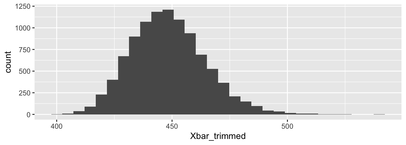
Figure 8.6: Bootstrap resampling estimate for the distribution of the trimmed mean.

Hypothesis testing is also possible with bootstrap methods, although we will only discuss the one sample test.

Given data \(x_1, \dotsc, x_n\), we want to test \(H_0: \mu = \mu_0\) against \(H_a: \mu \neq \mu_0\). We wish to estimate the sampling distribution of \(\overline{X}\) under the null hypothesis. One problem with using our data to do so is that the mean of our data is not \(\mu_0\)! The solution is to transform the data by adding \(\mu_0 - \overline{x}\) to each data point so that the mean of our data is \(\mu_0\):

\[ y_i = x_i + \mu_0 - \overline{x}. \]

By resampling \(y_i\), we get an estimate of the \(\overline{X}\) distribution under the null hypothesis. The \(p\)-value is then the proportion of the estimated distribution which is as extreme as the observed value \(\overline{x}\).

Example 8.33

Consider the weight_estimate data set in the fosdata package.

Image credit: Sciutti, et al..Image Credit
Sciutti, et al.. This is an open access article distributed under the terms of the Creative Commons Attribution License. https://journals.plos.org/plosone/article?id=10.1371/journal.pone.0224979

In this experiment,⁶¹ participants watched actors pick up objects of various weights, and then estimated the weight of the object. Let \(\mu\) be the mean value that a six-year-old child would estimate for the 200-gram object. We wish to test \(H_0: \mu = 200\) versus \(H_a: \mu \not= 200\). We start by examining the data. The histogram of mean200 is shown in Figure 8.7 with the hypothesized mean in blue and the sample mean in red.

weight <- fosdata::weight_estimate %>%
  filter(age == "6")
mean(weight$mean200)

## [1] 241.5789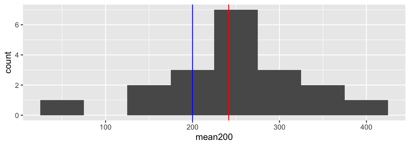

Figure 8.7: Six-year-old child estimates of the weight of a 200-gram object. Sample mean in red, hypothesized mean in blue.

The sample mean is 241.6 grams, which is higher than the value under \(H_0\). We now shift the data so it has mean 200 to match the null hypothesis.

weight_forboot <- weight$mean200 - mean(weight$mean200) + 200
mean(weight_forboot)

## [1] 200

We resample from this data and see how often we get a sample mean that is 241.6 or larger.

Xbar <- replicate(10000, {
  boot_weight <- sample(weight_forboot, replace = TRUE)
  mean(boot_weight)
})

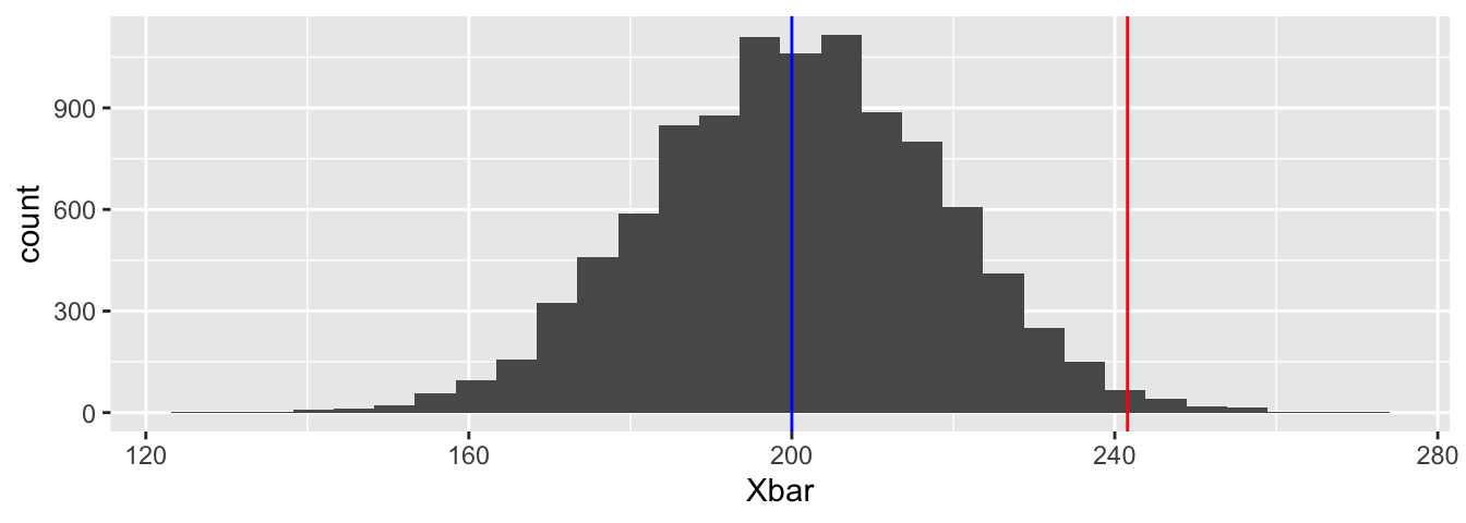
Figure 8.8: Bootstrap resampled distribution of mean weight estimates. Sample mean in red, hypothesized mean in blue.

Figure 8.8 shows the bootstrap resampled estimate for the distribution of \(\overline{X}\). It is unlikely, but not impossible, that the sample mean is 241.6. We can estimate the probability that \(\overline{X} \ge 241.6\) by computing⁶²

mean(Xbar >= mean(weight$mean200))

## [1] 0.0111

Since we are doing a two-sided test, we multiply by 2 to get the \(p\)-value.

2 * mean(Xbar >= mean(weight$mean200))

## [1] 0.0222

Since the \(p\)-value is less than 0.05, we reject the null hypothesis that the true mean weight estimate of six-year-olds is 200 grams. We get a similar result if we use t.test, though the \(p\)-value in t.test is somewhat higher.

t.test(weight$mean200, mu = 200)

## 
##  One Sample t-test
## 
## data:  weight$mean200
## t = 2.2456, df = 18, p-value = 0.03753
## alternative hypothesis: true mean is not equal to 200
## 95 percent confidence interval:
##  202.6782 280.4797
## sample estimates:
## mean of x 
##  241.5789

8.8.2 Permutation tests

Another popular resampling technique is the permutation test. If we imagine that there was no difference between two populations, then the assignments of the grouping variables can be considered random. A permutation test performs random permutations of the grouping variables, and re-computes the test statistic. Under \(H_0:\) “the response is independent of the grouping,” we should relatively frequently get values as extreme as the value obtained in the sample. We reject \(H_0\) if the proportion of times we get something as extreme as in the sample is less than \(\alpha\).

Let’s consider the masks data set in the fosdata package. The nasal_swab variable gives the viral load measured via a nasal swab for two types of influenza. We are interested in whether the mean viral loads are different in the two populations. Load the data with:

masks <- fosdata::masks

Next, we compute the mean viral load for virus type “A” minus the mean viral load for virus type “B.”

xbar_A <- masks %>%
  filter(pcr_type == "A") %>%
  pull(nasal_swab) %>%
  mean()
xbar_B <- masks %>%
  filter(pcr_type == "B") %>%
  pull(nasal_swab) %>%
  mean()
xbar_diff <- xbar_A - xbar_B
xbar_diff

## [1] -2484975

Type B had a larger viral load on average. Let’s look at a plot.

ggplot(masks, aes(x = pcr_type, y = nasal_swab)) +
  geom_boxplot(outlier.size = -1) +
  geom_jitter(height = 0, width = 0.2)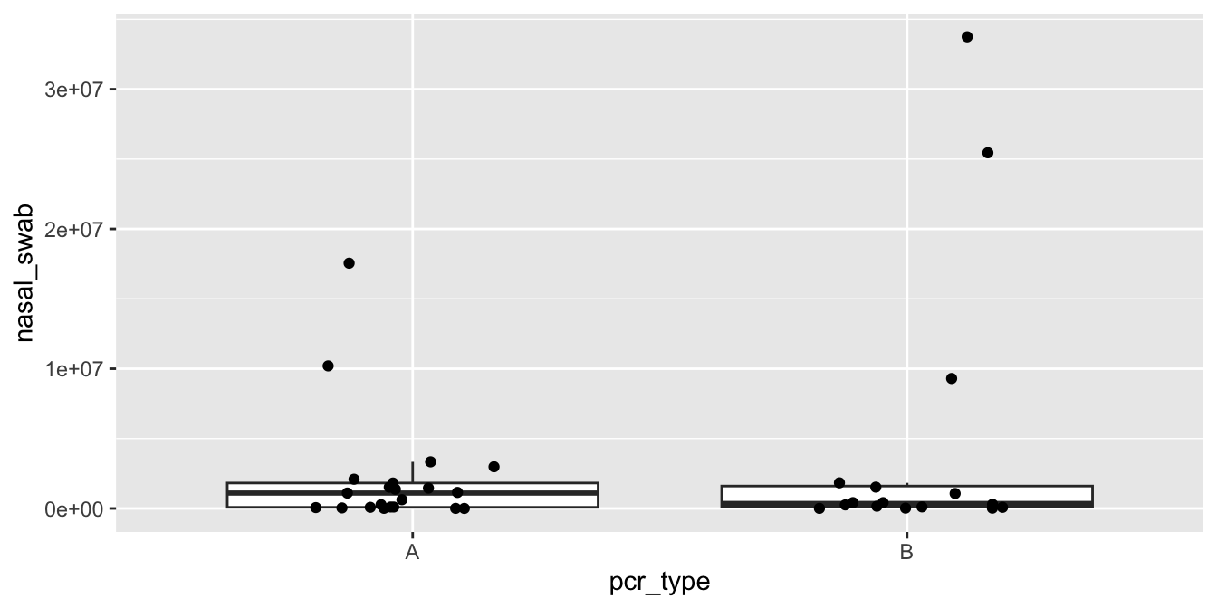

Figure 8.9: Viral load as measured by a nasal swab for two types of influenza.

The distribution in Figure 8.9 is visibly skewed, so there should be at least some hesitation to use a \(t\)-test. Instead, we permute the age groups many times and recompute the test statistic.

mu_diff <- replicate(10000, {
  # generate new randomly permuted age groups
  masks$permuted_type <- sample(masks$pcr_type)

  # recompute the difference in means
  mu_A <- masks %>%
    filter(permuted_type == "A") %>%
    pull(nasal_swab) %>%
    mean()
  mu_B <- masks %>%
    filter(permuted_type == "B") %>%
    pull(nasal_swab) %>%
    mean()
  mu_A - mu_B
})

data.frame(mu_diff) %>% ggplot(aes(x = mu_diff)) +
  geom_histogram() +
  geom_vline(xintercept = xbar_diff, color = "red")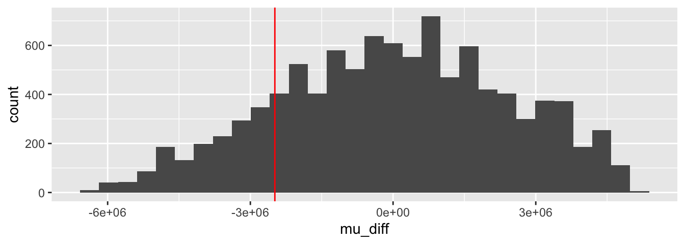

Figure 8.10: Difference in means for 10,000 permutations of the A and B groups. Observed value shown in red.

We see from the histogram (Figure 8.10) that it is not that unusual to get a value of -2484975. To get a \(p\)-value, we compute the percentage of resamples to the left (in Figure 8.10) of the observed value and double it.

2 * mean(mu_diff < xbar_diff)

## [1] 0.3328

We have a \(p\)-value of 0.3328, and we would not reject the null hypothesis. In the \(p\)-value computation, we only test for mu_diff < xbar_diff because xbar_diff is negative. For a positive observation, the inequality would reverse. We double it because we are performing a two-sided test.

Exercises

---

Exercises 8.1 – 8.5 require material through Section 8.1.

8.1

Let \(X_1, \ldots, X_{12}\) be independent normal random variables with mean 1 and standard deviation 3. Simulate 10000 values of \[ T = \frac{\overline{X} - 1}{S/\sqrt{12}} \] and plot the density function of \(T\). On your plot, add a curve in blue for \(t\) with 11 degrees of freedom. Also add a curve in red for the standard normal distribution. Confirm that the distribution of \(T\) is \(t\) with 11 df.

8.2

This exercise illustrates Theorem 8.1 in a specific instance. Let \(a = 0\) and \(b = 1\). Find the smallest value of \(n\) such that \(\left|P(a < X_n < b) - P(a < Z < b)\right| < .01\), where \(X_n\) is a \(t\) random variable with \(n\) degrees of freedom and \(Z\) is a standard normal random variable.

8.3

Let \(X\) be a \(t\) random variable with 6 degrees of freedom. Find a constant \(k > 0\) such that \[ P(-k < X < k) = .8 \]

8.4

Compute \(P(Z > 2)\), where \(Z\) is a standard normal random variable. Compute \(P(T > 2)\) for \(T\) having a \(t\) distribution with each of 40, 20, 10, and 5 degrees of freedom. How does the degrees of freedom affect the area in the tail of the \(t\) distribution?

8.5

Let \(X_1, \ldots, X_{20}\) be independent normal random variables with mean 7 and unknown standard deviation. Find the value of \(k\) such that \[ P(\overline{X} - k (S/ \sqrt{n}) < \mu < \overline{X} + k (S/ \sqrt{n})) = 0.99, \] where \(S\) as usual is the sample standard deviation.

---

Exercises 8.6 – 8.13 require material through Section 8.2.

8.6

The data set fosdata::plastics gives measurements of plastic microfibers found in snow. Give the 99% confidence interval for the mean diameter of plastic microfibers.

8.7

The data set morley is built into R. The Speed variable contains 100 measurements of the speed of light, conducted by A. A. Michelson in 1879. Measurements have 299000 km/s subtracted from them.

Compute the 95% confidence interval for the speed of light. Does your confidence interval contain the modern accepted speed of light of 299792 km/s?

8.8

Consider the fosdata::brake data set discussed in the chapter. Recall that latency_p2 is the time it takes subjects to release the pedal once they have pressed it and the car has started to accelerate rather than decelerate. Find a 95% confidence interval for the P2 latency for young drivers based on the data.

8.9

The data set fosdata::cows_small gives the change in shoulder temperature of cows standing in the heat.

1. Give the 95% confidence interval for the shoulder temperature change after spraying with the tk_12 nozzle.
2. Give the 95% confidence interval for the shoulder temperature change after no spraying (control).
3. Which of the two intervals is wider?
4. What is the standard deviation of temperature change for the tk_12 condition? For the control condition?
5. How are your answers to parts (c) and (d) related?

8.10

Suppose that \(X_1, \ldots, X_5\) is a random sample from a normal distribution with unknown mean and known standard deviation 2. If \(\overline{X} = 3\), then find a 95% confidence interval for the mean using the fact that \(\frac{\overline{X} - \mu}{\sigma/\sqrt{n}}\) is a standard normal random variable.

8.11

Some data randomly sampled from a normal population has a sample mean of 30. Match each interval on the left with one of the descriptions on the right:

Interval	Description
a. (28.5, 31.5)	I. 90% confidence interval.
b. (28.0, 32.0)	II. 95% confidence interval.
c. (28.7, 31.3)	III. 99% confidence interval.

8.12

Suppose you collect a random sample of size 20 from a normal population with unknown mean and standard deviation. Suppose \(\overline{x} = 2.3\) and \(s = 1.2\).

1. Find a 98% confidence interval for the mean.
2. The interval \((2.0, 2.6)\) is a confidence interval for the mean. What percent confidence interval is it?

8.13

Suppose a population has an exponential distribution with \(\lambda = 0.5\). We can simulate drawing a sample of size 10 from this population with rexp(10,0.5) and compute a 95% confidence interval with t.test(rexp(10,0.5),mu=2)$conf.int.

1. What is the population mean \(\mu\)?
2. Write code to simulate 10000 confidence intervals and determine what percent of the time \(\mu\) is in the 95% confidence interval.
3. Why is your answer different from 95%?

---

Exercises 8.14 – 8.19 require material through Section 8.3.

8.14

Consider the react data set from ISwR. Find a 98% confidence interval for the mean difference in measurements of the tuberculin reaction. Does the mean differ significantly from zero according to a \(t\)-test? Interpret.

8.15

The data fosdata::weight_estimate gives children’s estimates of weights lifted by actors (see Example 8.33). State and carry out a hypothesis test that the mean of the children’s estimates of the 100 g object differ from the actual weight, 100 g. Repeat this test for the 200, 300, and 400 g objects. Which of the estimates were significantly different from the correct weights?

8.16

Consider the bp.obese data set from ISwR. It contains data from a random sample of Mexican American adults in a small California town. Consider only the blood pressure data for this problem. Normal diastolic blood pressure is 120. Is there evidence to suggest that the mean blood pressure of the population differs from 120? What is the population in this example?

8.17

For the ISwR::bp.obese data set, consider the obese variable. What is the natural null hypothesis? Is there evidence to suggest that the obesity level of the population differs from the null hypothesis?

8.18

Suppose you collect a random sample of size 20 from a normal population with unknown mean and standard deviation. You wish to test \(H_0: \mu = 2\) versus \(H_a: \mu \not= 2\).

1. The region \(|T| > 1.6\) is a rejection region for this hypothesis test. What is the \(\alpha\) level of the rejection region?
2. Find a rejection region that corresponds to \(\alpha = 0.005\).

8.19

Suppose we wish to test \(H_0: \mu = 1\) versus \(H_a: \mu\not= 1\). Let \(X_1, \ldots, X_5\) be a random sample from a normal population with known standard deviation \(\sigma = 2\). We construct the test statistic \(Z = \frac{\overline{X} - 1}{\sigma/\sqrt{n}}\).

1. If the rejection region is \(|Z| > 2.2\), then what is the significance level of the test?
2. What would a rejection region be that corresponds to a significance level of \(\alpha = 0.01\)?

---

Exercise 8.20 requires material through Section 8.4.

8.20

Suppose that a dishonest statistician is doing a \(t\)-test of \(H_0: \mu = 0\) at the \(\alpha = 0.05\) level. The statistician waits until they get the data to specify the alternative hypothesis. If \(\overline{X} > 0\), then they choose \(H_a: \mu > 0\) and if \(\overline{X} < 0\), they choose \(H_a: \mu < 0\). Suppose the statistician collects 20 independent samples and the underlying population is standard normal. Use simulation to confirm that the null hypothesis is rejected 10% of the time.

---

Exercises 8.21 – 8.24 require material through Section 8.5.

8.21

This problem illustrates that t.test performs as expected when the underlying population is normal.

1. Choose 10 random values of \(X\) having the Normal(4, 1) distribution. Use t.test to compute the 95% confidence interval for the mean. Is 4 in your confidence interval?
2. Replicate the experiment in part (a) 10,000 times and compute the percentage of times the population mean 4 was included in the confidence interval.

8.22

Mackowiak et al.⁶³ studied the mean normal body temperature of healthy adults. One hundred forty-eight subjects’ body temperatures were measured one to four times daily for 3 consecutive days for a total of 700 temperature readings. Let \(\mu\) denote the true mean normal body temperature of healthy adults and \(X_1, \ldots, X_{700}\) the temperature readings from the study. Explain why \[ \frac{\overline{X} - \mu}{S/\sqrt{n}} \] is not a \(t\) random variable with 699 degrees of freedom.

8.23

This problem explores the accuracy of t.test when the underlying population is skewed.

1. Choose 10 random values of \(X\) having an exponential distribution with rate 1/4. Use t.test to compute the 95% confidence interval for the mean. Is the true mean, 4, in your confidence interval?
2. Replicate the experiment in part (a) 10,000 times and compute the percentage of times that the population mean 4 was included in the confidence interval. Explain why this number is not 95%.
3. Repeat part (b) using 100 values of \(X\) to make each confidence interval. What percentage of times did the confidence interval contain the population mean? Why is it closer to 95%?

8.24

This problem explores the accuracy of t.test when the data is not independent. Suppose \(X_1, \ldots, X_{20}\) is a random sample from normal population with mean 0 and standard deviation 1. Let \(Y_1 = X_1 + X_2\), \(Y_2 = X_2 + X_3, \ldots,\) and \(Y_{19} = X_{19} + X_{20}\). Note that \(Y_1, \ldots, Y_{19}\) are not independent, but they do have mean 0.

Estimate the effective type I error rate when testing \(H_0: \mu = 0\) versus \(H_a: \mu \not= 0\) at the \(\alpha = .05\) level using \(Y_1, \ldots, Y_{19}\).

(Hint: Y <- X[1:19]+X[2:20] computes \(Y\) as needed for this simulation.)

---

Exercises 8.25 – 8.40 require material through Section 8.6.

8.25

Each of these studies has won the prestigious Ig Nobel prize.⁶⁴ For each, state the null hypothesis.

1. Marina de Tommaso, Michele Sardaro, and Paolo Livrea, for measuring the relative pain people suffer while looking at an ugly painting, rather than a pretty painting, while being shot (in the hand) by a powerful laser beam.
2. Atsuki Higashiyama and Kohei Adachi, for investigating whether things look different when you bend over and view them between your legs.
3. Patricia Yang, David Hu, Jonathan Pham, and Jerome Choo, for testing the biological principle that nearly all mammals empty their bladders in about 21 seconds.

8.26

The didgeridoo is an Indigenous Australian musical instrument. In a 2006 study⁶⁵ that recently won the Ig Nobel Peace Prize, researchers investigated didgeridoo playing as a treatment for sleep apnoea, a breathing disorder that interferes with sleep. The researchers separated 25 patients into a treatment group that received didgeridoo lessons and a control group that did not. From the paper:

Participants in the didgeridoo group practiced an average of 5.9 days a week (SD 0.86) for 25.3 minutes (SD 3.4). Compared with the control group in the didgeridoo group daytime sleepiness (difference -3.0, 95% confidence interval -5.7 to -0.3, \(P = 0.03\)) and apnoea-hypopnoea index (difference -6.2, -12.3 to -0.1, \(P = 0.05\)) improved significantly and partners reported less sleep disturbance (difference -2.8, -4.7 to -0.9, \(P < 0.01\)). There was no effect on the quality of sleep (difference -0.7, -2.1 to 0.6, \(P = 0.27\)). The combined analysis of sleep related outcomes showed a moderate to large effect of didgeridoo playing.

1. The paper reports four measurements. All four differences are reported as negative numbers. What does that tell you?
2. Only one of their reported measures did not show a significant improvement for the didgeridoo group. Which one? How do you know it was not significant?
3. Which of their reported measures was the most significant evidence in favor of didgeridoo playing?

8.27

The data set fosdata::chimps was introduced in Example 7.8. The variable grey_score_avg is a measurement of the grey hair in chimpanzees in the study. Two subspecies of chimps are in this study: verus and schweinfurthii. Is there evidence at the \(\alpha = 0.05\) level to suggest that the mean grey score differs between the two subspecies?

8.28

Experimenters measured the leg strength of adults using two methods: a stationary isometric dynamometer and a Wii Balance Board. The strength (in kg) of each adult is reported in fosdata::leg_strength.

Test for a difference in the mean leg strength as measured with these two devices.

8.29

The data set cigs from the fosdata package contains measurements of cigarette brands that were tested by the U.S. Federal Trade Commission for chemical content. Check with a plot that the nicotine (nic) and tar variables are reasonably bump shaped and symmetric, without major outliers.

1. Test for a difference in nicotine content between filtered and unfiltered cigarette brands. State your result with a \(p\)-value.
2. Test for a difference in tar content between filtered and unfiltered cigarette brands. State your result with a \(p\)-value.
3. Test for a difference in nicotine content between menthol and non-menthol cigarette brands. State your result with a \(p\)-value.
4. Test for a difference in tar content between menthol and non-menthol cigarette brands. State your result with a \(p\)-value.

8.30

For the ISwR::bp.obese data set from Exercise 8.16, is there evidence to suggest that the mean blood pressure of Mexican American men is different from that of Mexican American women in this small California town? Would it be appropriate to generalize your answer to the mean blood pressure of men and women in the USA?

8.31

Consider the ex0112 data in the Sleuth3 package. The researchers randomly assigned 7 people to receive fish oil and 7 people to receive regular oil, and measured the decrease in their diastolic blood pressure. Is there sufficient evidence to conclude that the mean decrease in blood pressure of patients taking fish oil is different from the mean decrease in blood pressure of those taking regular oil?

8.32

The barnacles data in fosdata has measurements of barnacle density on various coral reefs. Some reefs are considered deep and some shallow, as given by the deep variable. For this exercise, only consider the reefs with location FGB, the Flower Garden Banks in the Gulf of Mexico.

1. Check that barnacle_density is right-skewed, but that the log of barnacle_density is close to normally distributed.
2. Perform a two sample \(t\)-test to determine if the log of barnacle_density is different for deep and shallow reefs. Report your results with a \(p\)-value.

8.33

Consider the ex0333 data in the Sleuth3 package. This is an observational study of brain size and litter size in mammals. Create a boxplot of the brain size for large litter and small litter mammals. Does the data look normal? Create a histogram or a qq plot. Repeat after taking the logs of the brain sizes. Is there evidence to suggest that there is a difference in mean brain sizes of large litter animals and small litter animals?

8.34

Consider the case0202 data in the Sleuth3 package. This data is from a study of twins, where one twin was schizophrenic and the other was not. The researchers used magnetic resonance imaging to measure the volumes (in \(\text{cm}^3\)) of several regions and subregions of the twins’ brains. State and carry out a hypothesis test that there is a difference in the volume of these brain regions between the Affected and the Unaffected twins.

8.35

Consider the cows_small data set in the fosdata package that was discussed in this chapter.

1. Is there sufficient evidence to conclude that the mean temperature change associated with the TK-12 nozzle is less than the mean temperature change associated with not spraying the cows at all; that is, with the control?

2. Is there sufficient evidence to conclude that the mean temperature change associated with the TK-12 nozzle is different than the mean temperature change associated with the TK-0.75 nozzle?

---

The next exercises use the data set fosdata::child_tasks, which comes from a study by Chan and Morgan⁶⁶ that studies the length of time needed for children to complete various tasks.

8.36

Consider the child_tasks data set in the fosdata package. Let \(\mu_1\) be the mean time for girls to finish the day night task, and let \(\mu_2\) be the mean time for boys to finish the same task. Perform a two-sided hypothesis test of \(H_0: \mu_1 = \mu_2\) at the \(\alpha = .01\) level.

8.37

Consider the child_tasks data set in the fosdata package. It seems likely that age of participant is an important factor in the length of time the children take to perform tasks. Since the sampling method for obtaining participants might not be a true random sample, we might wonder whether the mean age of boys and girls via the sampling method for this experiment are the same. Let \(\mu_1\) be the mean age for girls and let \(\mu_2\) be the mean age for boys. Perform a two-sided hypothesis test of \(H_0: \mu_1 = \mu_2\) at the \(\alpha = .05\) level.

8.38

Consider the child_tasks data set in the fosdata package. Let \(\mu_1\) be the mean time for children in the 7 year old group to finish the day night task, and let \(\mu_2\) be the mean time for children in the 6 year old group to finish the same task. Perform a two-sided hypothesis test of \(H_0: \mu_1 = \mu_2\) at the \(\alpha = .01\) level.

8.39

Consider the child_tasks data set in the fosdata package. The “card sort” task asks children to sort cards either by the shape pictured on the card or the color of that shape. They first do one task, then switch to the other task. Children’s times at these tasks are recorded in the card_sort_preswitch_time_secs and card_sort_postswitch_time_secs variables.

Let \(\mu_1\) be the mean time for the pre-switch task and \(\mu_2\) be the mean time for the post-switch task. Perform a two-sided hypothesis test of \(H_0: \mu_1 = \mu_2\) at the \(\alpha = .01\) level. Are the children faster pre- or post-switch?

8.40

Example 8.21 tested the difference in latency_p2 times between young and older subjects, with data from fosdata::brake. Repeat the analysis with the largest older outlier removed. Does removing the largest older outlier change the conclusion of your test at the \(\alpha = .05\) level?

---

Exercises 8.41 – 8.50 require material through Section 8.7.

8.41

In a jury trial, the null hypothesis is that the defendant is innocent (“presumed innocent until proven guilty”). The alternate hypothesis is that the defendant is guilty.

1. If the defendant actually committed the crime but is found not guilty, what type of error is that?
2. If the defendant is innocent but is found guilty, what type of error is that?
3. In your opinion, which type of error is more serious, and why?

8.42

In a drug trial, patients are given a drug to test if it will cure their illness.

1. What is the null hypothesis for a drug trial?
2. What would a type I error be for a drug trial?
3. What would a type II error be for a drug trial?
4. What are the implications for each type of error for ill patients?
5. What are the implications for each type of error for drug manufacturers?

8.43

Suppose you wish to test the side effects of a new vaccine by forming two groups of subjects, one that gets the vaccine and another that gets a placebo. You would like to detect a \(1^\circ F\) change in body temperature at the \(\alpha = 0.05\) level of significance with a power of 99%. Data on human body temperature (such as fosdata::normtemp) suggests that the standard deviation of body temperature is around \(0.73^\circ F\). How many subjects will you need in each group?

8.44

The compressive strength of concrete is the pressure (N/mm\(^2\)) at which it fails. The compressive strength of a particular type of concrete follows a \(\text{Norm}(65, 6)\) distribution. When concrete is poured at a construction site, five cubes are poured and taken to a lab for testing. Suppose the actual concrete pour has a mean compressive strength of only 60. What power does this test have to detect the difference in means? Use a \(0.05\) significance level.

8.45

Suppose a population has mean 0 and standard deviation \(\sqrt{3}\). We want to test the (false) null hypothesis \(H_0: \mu = 1\) with a sample size of \(n = 40\) and \(\alpha = 0.05\).

1. Suppose the population is \(\text{Norm}(0,\sqrt{3})\). What is the power of a \(t\)-test to detect this difference in means?
2. Suppose the population is \(t\) with 3 degrees of freedom, which has standard deviation \(\sqrt{3}\). Perform a simulation to determine the power of the \(t\)-test to detect the difference in means.

8.46

The purpose of this exercise is to examine the effect of sample size, effect size, and significance level on the power of a test.

1. Fix an effect size of \(d = 0.2\) and a significance level of \(\alpha = 0.05\), and compute the power of a two-sided one sample \(t\)-test for \(n = 200\) and \(n = 400\). What happens to the power?
2. Fix a significance level of \(\alpha = 0.05\) and \(n = 200\), and compute the power of a two-sided one sample \(t\)-test for \(d = 0.2\) and \(d = 0.4\). What happens to the power?
3. Fix \(n = 200\) and an effect size of \(d = 0.2\), and compute the power of a two-sided one sample \(t\)-test for \(\alpha = 0.05\) and \(\alpha = 0.1\). What happens to the power?

---

The next two exercises use the data set fosdata::wrist, which comes from a study by Raittio et al.⁶⁷ that considers two different methods for applying casts to wrist fractures.

8.47

The authors performed a power analysis in order to determine sample size. They wanted a power of 80% at the \(\alpha = .05\) level, and they assumed that 30% of their patients would drop out. Previous studies had shown that the standard deviation of the prwe12m variable would be about 14. They concluded that they needed 40 participants in each group. What difference in means did they use in their power computation? (You can check your answer by looking up their paper.)

8.48

The authors used the fosdata::wrist data set to find a 95% confidence interval for the difference in the mean of prwe12m between the functional cast position and the volar-flexion and ulnar deviation cast position. They assumed equal variances in the two populations to find the 95% confidence interval.

1. Find the 95% confidence interval of the mean difference assuming equal variances.
2. Compare your answer to the result in the published paper.
3. Was assuming equal variance justified?

8.49

This exercise explores how the \(t\)-test changes when data values are transformed.

1. Suppose you wish to test \(H_0: \mu = 0\) versus \(H_a: \mu \not = 0\) using a \(t\)-test. You collect data \(x_1 = -1,x_2 = 2,x_3 = -3,x_4 = -4\) and \(x_5 = 5\). What is the \(p\)-value?
2. Now, suppose you multiply everything by 2: \(H_0: \mu = 0\) versus \(H_a: \mu\not = 0\) and your data is \(x_1 = -2\), \(x_2 = 4\), \(x_3 = -6\), \(x_4 = -8\), and \(x_5 = 10\). What happens to the \(p\)-value? (Try to answer this without using R. Check your answer using R, if you must.)
3. Now, suppose you square the magnitudes of everything. \(H_0: \mu = 0\) versus \(H_a: \mu \not= 0\), and your data is \(x_1 = -1\), \(x_2 = 4\), \(x_3 = -9\), \(x_4 = -16\), and \(x_5 = 25\). What happens to the \(p\)-value?

8.50

This problem explores how the \(t\)-test behaves in the presence of an outlier.

1. Create a data set of 20 random values \(x_1,\ldots,x_{20}\) with a normal distribution with mean 10 and sd 1. Replace \(x_{20}\) with the number 1000. Perform a \(t\)-test with \(H_0 : \mu = 0\), and observe the value of \(t\). It should be close to 1. Is the \(t\)-test able to find a significant difference between the mean of this data and 0?

   The next parts of this problem ask you to prove that the \(t\)-test statistic is always close to 1 in the presence of a large outlier.

2. Assume that \(x_1,\ldots,x_{n-1}\) are not changing, but \(x_n\) varies. Let \(\overline{x} = \frac 1n \sum_{i=1}^n x_i\) as usual. Show that \[ \lim_{x_n\to\infty} \frac{\overline{x}}{x_n} = \frac{1}{n}. \]

3. Let the sample variance be \(s^2 = \frac 1{n-1}\sum_{i=1}^n (x_i - \overline{x})^2\) as usual. Show that \[ \lim_{x_n\to\infty} \frac{s^2}{x_n^2} = \frac{1}{n}. \]

4. Finally show that \[ \lim_{x_n\to\infty} \frac{\overline{x} - \mu_0}{s/\sqrt{n}} = 1, \] where \(\mu_0\) is any real number. (Hint: divide top and bottom by \(x_n\), then use parts (b) and (c)).

5. What does this say about the ability of a \(t\)-test to reject \(H_0: \mu = \mu_0\) at the \(\alpha = .05\) level as \(x_n\to \infty\)?

---

Exercises 8.51 – 8.55 require material through Section 8.8.

8.51

Consider the weight_estimate data from the fosdata package. Construct a bootstrap 95% confidence interval for the true mean weight that adults estimate for the 400-gram object.

8.52

Consider the masks data from the fosdata package. Thirty-seven patients with confirmed influenza were given nasal swabs and the viral load was computed in the variable nasal_swab. Our goal is to use this data to make a 95% confidence interval for the mean viral load in influenza patients.

1. Is it appropriate to use a the \(t\) statistic and t.test to make a 95% confidence interval? Explain.
2. Create a bootstrap 95% confidence interval for the true mean viral load for influenza patients.

8.53

Consider the brake data from the fosdata package. Construct a bootstrap 95% confidence interval for the median of the latency_p1 variable for older drivers.

8.54

Consider the react data from the ISwR package. Construct a bootstrap 98% confidence interval for the true mean difference in estimates of reaction size.

8.55

The data set morley is built into R. The Speed variable contains 100 measurements of the speed of light, conducted by A. A. Michelson in 1879. Measurements have 299000 km/s subtracted from them.

The currently accepted speed of light is 299792 kilometers/second. Perform a bootstrap hypothesis test at the \(\alpha = .05\) level of \(H_0: \mu = 792\) versus \(H_a: \mu\not= 792\).

---

52. K Hasegawa, M Kimura, and Y Takeda, “Age-Related Differences in Correction Behavior for Unintended Acceleration,” PLOS One 15, no. 7 (2020): e0236053, https://doi.org/10.1371/journal.pone.0236053.↩︎

53. This data is derived from a data set presented in P Mackowiak, S Wasserman, and M Levine, “A Critical Appraisal of 98.6 Degrees F, the Upper Limit of the Normal Body Temperature, and Other Legacies of Carl Reinhold August Wunderlich.” JAMA 268 12 (1992): 1578–80. Data was constructed to match as closely as possible the histograms and summary statistics presented in that article. Additional information about this data set can be found in L Shoemaker Allen, “What’s Normal? – Temperature, Gender, and Heart Rate,” Journal of Statistics Education 4, no. 2 (1996), https://doi.org/10.1080/10691898.1996.11910512.↩︎

54. This example and a thought provoking examination of related issues can be found in Richard D Morey et al., “The Fallacy of Placing Confidence in Confidence Intervals,” Psychonomic Bulletin & Review 23, no. 1 (2016): 103–23, https://doi.org/10.3758/s13423-015-0947-8.↩︎

55. C A Wunderlich and W B Woodman, On the Temperature in Diseases: A Manual of Medical Thermometry, New Sydenham Society Publications (New Sydenham Society, 1871).↩︎

56. Jennifer Van Os, Karin Schutz, and Cassandra Tucker, “Cooling Cows Efficiently with Sprinklers: Physiological Responses to Water Spray,” Journal of Dairy Science 98 (July 2015), https://doi.org/10.3168/jds.2015-9434.↩︎

57. With human subjects, the control group usually receives a placebo treatment so that the subjects and experimenters are unaware (blind) of which group they are in.↩︎

58. We say the outlier is extreme because if we run boxplot(rnorm(40, 956, 242)), it is extremely rare to see an outlier that is so far away from the mean.↩︎

59. When the standard deviation of a population is unknown, it is often easier to estimate the range of possible values and divide by 4 or 6 to get a rough estimate of the standard deviation.↩︎

60. Bradley Efron and Robert J Tibshirani, An Introduction to the Bootstrap, Monographs on Statistics and Applied Probability 57 (New York: Chapman & Hall, 1993).↩︎

61. Alessandra Sciutti, Laura Patanè, and Giulio Sandini, “Development of Visual Perception of Others’ Actions: Children’s Judgment of Lifted Weight,” PLOS One 14, no. 11 (November 2019): e0224979.↩︎

62. It can be argued that we should count the data that we obtained as one of the bootstrap samples and estimate the \(p\)-value via 2 * (sum(Xbar >= mean(weight$mean200)) + 1)/10001. One advantage of this is that it prevents an estimated \(p\)-value of exactly 0.↩︎

63. Mackowiak, Wasserman, and Levine, “A Critical Appraisal of 98.6 Degrees F, the Upper Limit of the Normal Body Temperature, and Other Legacies of Carl Reinhold August Wunderlich.”↩︎

64. See https://www.improbable.com/ig/↩︎

65. Milo A Puhan et al., “Didgeridoo Playing as Alternative Treatment for Obstructive Sleep Apnoea Syndrome: Randomised Controlled Trial,” BMJ: British Medical Journal 332, no. 7536 (2006): 266–68.↩︎

66. Amy Y C Chan and Sarah-Jane Morgan, “Assessing Children’s Cognitive Flexibility with the Shape Trail Test.” PLOS One 13, no. 5 (2018): e0198254.↩︎

67. Lauri Raittio et al., “Two Casting Methods Compared in Patients with Colles’ Fracture: A Pragmatic, Randomized Controlled Trial,” PLOS One 15, no. 5 (May 2020): e0232153.↩︎