Probability, Statistics, and Data: A Fresh Approach Using R

Chapter 1 Data in R

The R Statistical Programming Language plays a central role in this book. While there are several other programming languages and software packages that do similar things, we chose R for several reasons:

R is widely used among statisticians, especially academic statisticians. If there is a new statistical procedure developed somewhere in academia, chances are that the code for it will be made available in R. This distinguishes R from, say, Python.
R is commonly used for statistical analyses in many disciplines. Other software, such as SPSS or SAS is also used and in some disciplines would be the primary choice for some discipline specific courses, but R is popular and its user base is growing.
R is free. You can install it and all optional packages on your computer at no cost. This is a big difference between R and SAS, SPSS, MATLAB, and most other statistical software.
R has been experiencing a renaissance. With the advent of the tidyverse and RStudio, R is a vibrant and growing community. We also have found the community to be extremely welcoming. The R ecosystem is one of its strengths.

In this chapter, we will begin to see some of the capabilities of R. We point out that R is a fully functional programming language, as well as being a statistical software package. We will only touch on the nuances of R as a programming language in this book.

1.1 Arithmetic and variable assignment

We begin by showing how R can be used as a calculator. Here is a table of commonly used arithmetic operators.

Table 1.1: Basic arithmetic operators in R.
Operator	Description	Example
`+`	addition	`1 + 1`
`-`	subtraction	`4 - 3`
`*`	multiplication	`3 * 7`
`/`	division	`8 / 3`
`^`	exponentiation	`2^3`

The output of the examples in Table 1.1 is given below. Throughout the book, lines that start with ## indicate output from R commands. These will not show up when you type in the commands yourself. The [1] in the lines below indicate that there is one piece of output from the command. These will show up when you type in the commands.

1 + 1

## [1] 2

4 - 3

## [1] 1

3 * 7

## [1] 21

8 / 3

## [1] 2.666667

2^3

## [1] 8

A couple of useful constants in R are pi and exp(1), which are $\pi \approx 3.141593$ and $e \approx 2.718282.$ Here R a couple of examples of how you can use them.

pi^2

## [1] 9.869604

2 * exp(1)

## [1] 5.436564

R is a functional programming language. If you don’t know what that means, that’s OK, but as you might guess from the name, functions play a large role in R. We will see many, many functions throughout the book. Every time you see a new function, think about the following four questions:

What type of input does the function accept?
What does the function do?
What does the function return as output?
What are some typical examples of how to use the function?

In this section, we focus on functions that do things that you are likely already familiar with from your previous math courses.

We start with exp. The function exp takes one argument named x and returns $e^x$. So, for example, exp(x = 1) will compute $e^1 = e$, as we saw above. In R, it is optional as to whether you supply the named version x = 1 or just 1 as the argument. So, it is equivalent to write exp(x = 1) or exp(1). Typically, for functions that are “well-known,” the first argument or two will be given without names, then the rest will be provided with their names. Our advice is that if in doubt, include the name.

Next, we discuss the log function. The function log takes two arguments x and base and returns $\log_{b}x$, where $b$ is the base. The x argument is required. The base argument is optional with a default value of $e$. In other words, the default logarithm is the natural logarithm. Here are some examples of using exp and log.

exp(2)

## [1] 7.389056

log(8)

## [1] 2.079442

log(8, base = 2)

## [1] 3

You can’t get very far without storing results of your computations to variables! The way¹ to do so is with the arrow <-. Typing Alt + - is the keyboard shortcut for <-.

height <- 62 # in inches
height <- height + 2
height <- 3 * height

The # in inches part of the code above is a comment. These are provided to give the reader information about what is going on in the R code, but are not executed and have no impact on the output.

If you want to see what value is stored in a variable, you can

type the variable name

height

## [1] 192

look in the environment box in the upper right-hand corner of RStudio.
Use the str command. This command gives other useful information about the variable, in addition to its value.

str(height)

##  num 192

This says that height contains num-eric data, and its current value is 192 (which is 3(62 + 2)). Note that there is a big difference between typing height + 2 (which computes the value of height + 2 and displays it on the screen) and typing height <- height + 2, which computes the value of height + 2 and stores the new value back in height.

Alert 1.1

It is important to choose your variable names wisely. Variables in R cannot start with a number, and for our purposes, they should not start with a period. Do not use T or F as a variable name. Think twice before using c, q, t, C, D, or I as variable names, as they are already defined. It may also be a bad idea (and is one of the most frustrating things to debug on the rare occasions that it causes problems) to use sum, mean, or other commonly used functions as variable names. T and F are variables with default values TRUE and FALSE, which can be changed. We recommend writing out TRUE and FALSE rather than using the shortcuts T and F for this reason.

We also misspoke when we said pi is a constant. It is actually a variable which is set to 3.141593 when R is started, but can be changed to any value you like.² If you find that pi or T or F has been changed from a default, and you want to have them return to the default state, you have a couple of choices. You can restart R by clicking on Session/Restart. This will do more than just reset variables to their default values; it will reset R to its start-up state. Or, you can remove a variable from the R environment by using the function rm(). The function rm accepts the name of a variable and removes it from memory. As an example, look at the code below:

pi

## [1] 3.141593

pi <- 3.2
pi

## [1] 3.2

rm(pi)
pi

## [1] 3.141593

We end this section with a couple more hints. To remove all of the variables from your working environment, click on the broom icon in the Environment tab in RStudio. You may want to do this from time to time, as R can slow down when it has too many large variables in the current environment.

If you have a longish variable name in your environment, then you can use the tab key to auto-complete. Finally, RStudio has an option to restore the data in your working environment when you restart R. We recommend turning this off by going to RStudio -> Preferences and unchecking the box “Restore .RData into workspace at startup.” This will ensure that each time you start R, all of the commands that you used to create the data in your environment will be run inside that R session.

1.2 Help

R comes with built-in help. In RStudio, there is a help tab in the lower right pane. From the console, placing a ? before an object gives help for that object.

Tryit 1.1

Type ?log in the console to see the help page for log and exp.

Help pages in R have some standard headings. Let’s look at some of the main areas in the help page for log.

Description: The help page says that log computes logarithms, by default natural logarithms.
Usage: log(x, base = exp(1)) means that log takes two arguments, x and base, and that base has a default of exp(1).
Arguments: x is a numeric or complex vector, and base is a positive or complex number. This might be confusing for now, because we indicated that x was a positive real number above, but the help page indicates that log is more flexible than what we have seen so far.
Examples: The help page provides code that you can copy and paste into the R console to see what the function does. In this case, it provides among other things, log(exp(3)), which is equal to 3.

It can take some time to get used to reading R Documentation. For now, we recommend reading those four headings to see whether there are things you can learn about new functions. Don’t worry if there are things in the documentation that you don’t yet understand.

1.3 Vectors

Data often takes the form of multiple values of the same type. In R, multiple values are stored in a data type called a vector. R is designed to work with vectors quickly and easily.

There are many ways to create vectors. Perhaps the easiest is the c function:

c(2, 3, 5, 7, 11)

## [1]  2  3  5  7 11

The c function combines the values given to it into a vector. In this case, the vector is the list of the first 5 prime numbers. We can store vectors in variables just like we did with numbers:

primes <- c(2, 3, 5, 7, 11)

You can also create a vector of numbers in order using the : operator:

1:10

##  [1]  1  2  3  4  5  6  7  8  9 10

The rep function is a more flexible way of creating vectors. It has a required argument x, which is a vector of values that are to be repeated (could be a single value as well). It has optional arguments times, length.out and each. Normally, just one of the additional arguments is specified, and we will not discuss what happens if multiple arguments are specified. The argument times specifies the number of times that the value in x is repeated. This can either be specified as a single value, in which case the values of x are repeated that many times, or as a vector of values the same length as x. In this case, the values in x are repeated the number of times associated with the vector, but the ordering is different. For example:

rep(c(2, 3), times = 2)

## [1] 2 3 2 3

rep(c(2, 3), times = c(2, 2))

## [1] 2 2 3 3

rep(c(2, 3), times = c(2, 3))

## [1] 2 2 3 3 3

Alternatively, you can specify the length of the vector that you are trying to obtain, using length.out. R will truncate the last repetition of the vector that you are repeating to force the length to be exactly length.out.

rep(c(2, 3), length.out = 6)

## [1] 2 3 2 3 2 3

rep(c(2, 3), length.out = 3)

## [1] 2 3 2

Finally, setting each to a number repeats each value in x the same number of times. However, it orders the values as if you had written a vector of values in times.

rep(c("Bryan", "Darrin"), each = 2)

## [1] "Bryan"  "Bryan"  "Darrin" "Darrin"

rep(c("Bryan", "Darrin"), times = 2)

## [1] "Bryan"  "Darrin" "Bryan"  "Darrin"

We see here that the original vector x does not have to be numeric!

One last useful function for creating vectors is seq. This is a generalization of the : operator described above. We will not go over the entire list of arguments associated with seq, but we note that it has arguments from, to, by and length.out. We provide a couple of examples that we hope illustrate well enough how to use seq.

seq(from = 1, to = 11, by = 2)

## [1]  1  3  5  7  9 11

seq(from = 1, to = 11, length.out = 21)

##  [1]  1.0  1.5  2.0  2.5  3.0  3.5  4.0  4.5  5.0  5.5  6.0  6.5  7.0
## [14]  7.5  8.0  8.5  9.0  9.5 10.0 10.5 11.0

Once you have created a vector, you may also want to do arithmetic or other operations on it. Most of the operations in R work “as expected” with vectors. Suppose you wanted to see what the square roots of the first 5 primes were. You might guess:

primes^(1 / 2)

## [1] 1.414214 1.732051 2.236068 2.645751 3.316625

and you would be right! Returning to the cryptic manual entry in log, we recall that it stated that x is a numeric vector. This is the documentation’s way of telling us that log is vectorized. If we supply the log function with a vector of values, then log will compute the log of each value separately. For example,

log(primes)

## [1] 0.6931472 1.0986123 1.6094379 1.9459101 2.3978953

Other commands reduce a vector to a number, for example sum adds all elements of the vector, and max finds the largest.

sum(primes)

## [1] 28

max(primes)

## [1] 11

Tryit 1.2

Guess what would happen if you type primes + primes, primes * primes and sum(1/primes). Were you right?

The plot command creates graphic images from data. This book will only use plot for simple graphics, preferring the more powerful ggplot command discussed in Chapter 7. In its most basic application, give plot vectors of $x$- and $y$-coordinates, and it will produce a graphic with a point shown for each $(x,y)$ pair.

x <- -10:10
y <- x^2
plot(x, y)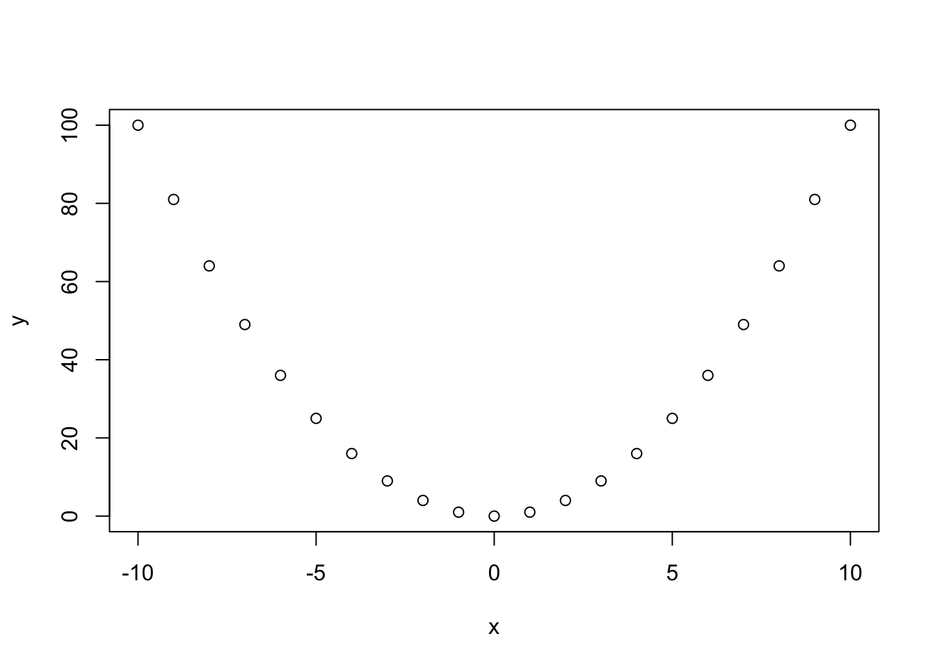

1.4 Indexing vectors

To examine or use a single element in a vector, you need to supply its index. primes[1] is the first element in the vector of primes, primes[2] is the second, and so on.

primes[1]

## [1] 2

primes[2]

## [1] 3

You can do many things with indexes. For example, you can provide a vector of indices, and R will return a new vector with the values associated with those indices.

primes[1:3]

## [1] 2 3 5

You can remove a value from a vector by using a - sign.

primes[-1]

## [1]  3  5  7 11

You can provide a vector of TRUE and FALSE values as an index, and R will return the values that are associated with TRUE. As a beginner, take care to have the length of the vector of TRUE and FALSE values be the same length as the original vector.

primes[c(TRUE, FALSE, TRUE, FALSE, TRUE)]

## [1]  2  5 11

The construct of providing a Boolean vector (that is, a vector containing TRUE and FALSE) for indexing is most useful for selecting elements that satisfy some condition. Suppose we wanted to “pull out” the values in primes that are bigger than 6. We create an appropriate vector of TRUE and FALSE values, then index primes by it.

primes > 6

## [1] FALSE FALSE FALSE  TRUE  TRUE

primes[primes > 6]

## [1]  7 11

Observe the use of > for comparison. In R (and most modern programming languages), there are some fundamental comparison operators:

== equal to
!= not equal to
> greater than
< less than
>= greater than or equal to
<= less than or equal to

Another important operator is the %in%, which is TRUE if a value is in a vector. For example:

4 %in% primes

## [1] FALSE

odds <- seq(from = 1, to = 11, by = 2)
primes[primes %in% odds]

## [1]  3  5  7 11

R comes with many built-in data sets. For example, the rivers data set is a vector containing the length of major North American rivers. Try typing ?rivers to see some more information about the data set. Let’s see what the data set contains.

rivers

##   [1]  735  320  325  392  524  450 1459  135  465  600  330  336  280
##  [14]  315  870  906  202  329  290 1000  600  505 1450  840 1243  890
##  [27]  350  407  286  280  525  720  390  250  327  230  265  850  210
##  [40]  630  260  230  360  730  600  306  390  420  291  710  340  217
##  [53]  281  352  259  250  470  680  570  350  300  560  900  625  332
##  [66] 2348 1171 3710 2315 2533  780  280  410  460  260  255  431  350
##  [79]  760  618  338  981 1306  500  696  605  250  411 1054  735  233
##  [92]  435  490  310  460  383  375 1270  545  445 1885  380  300  380
## [105]  377  425  276  210  800  420  350  360  538 1100 1205  314  237
## [118]  610  360  540 1038  424  310  300  444  301  268  620  215  652
## [131]  900  525  246  360  529  500  720  270  430  671 1770

By typing ?rivers, we learn that this data set gives the lengths (in miles) of 141 major rivers in North America, as compiled by the US Geological Survey. This data set is explored further in the exercises in this chapter. We will often want to examine only the first few elements when the data set is large. For that, we can use the function head, which by shows the first six elements.

head(rivers)

## [1] 735 320 325 392 524 450

The discoveries data set is a vector containing the number of “great” inventions and scientific discoveries in each year from 1860 to 1959. Try ?discoveries to see more information about the discoveries data set. You might try the examples listed there just to see what they do, but we won’t be doing anything like that yet. Let’s see what the data set contains.

discoveries

## Time Series:
## Start = 1860 
## End = 1959 
## Frequency = 1 
##   [1]  5  3  0  2  0  3  2  3  6  1  2  1  2  1  3  3  3  5  2  4  4  0
##  [23]  2  3  7 12  3 10  9  2  3  7  7  2  3  3  6  2  4  3  5  2  2  4
##  [45]  0  4  2  5  2  3  3  6  5  8  3  6  6  0  5  2  2  2  6  3  4  4
##  [67]  2  2  4  7  5  3  3  0  2  2  2  1  3  4  2  2  1  1  1  2  1  4
##  [89]  4  3  2  1  4  1  1  1  0  0  2  0

If we type str(discoveries) we see that the data set is stored as a time series rather than as a vector. For our purposes in this section, that will be an unimportant distinction, and we can simply think of the variable as a vector of numeric values.

The first ten elements are:

head(discoveries, n = 10)

##  [1] 5 3 0 2 0 3 2 3 6 1

Here are a few more things you can do with a vector:

sort(discoveries)

##   [1]  0  0  0  0  0  0  0  0  0  1  1  1  1  1  1  1  1  1  1  1  1  2
##  [23]  2  2  2  2  2  2  2  2  2  2  2  2  2  2  2  2  2  2  2  2  2  2
##  [45]  2  2  2  3  3  3  3  3  3  3  3  3  3  3  3  3  3  3  3  3  3  3
##  [67]  3  4  4  4  4  4  4  4  4  4  4  4  4  5  5  5  5  5  5  5  6  6
##  [89]  6  6  6  6  7  7  7  7  8  9 10 12

sort(discoveries, decreasing = TRUE)

##   [1] 12 10  9  8  7  7  7  7  6  6  6  6  6  6  5  5  5  5  5  5  5  4
##  [23]  4  4  4  4  4  4  4  4  4  4  4  3  3  3  3  3  3  3  3  3  3  3
##  [45]  3  3  3  3  3  3  3  3  3  2  2  2  2  2  2  2  2  2  2  2  2  2
##  [67]  2  2  2  2  2  2  2  2  2  2  2  2  2  1  1  1  1  1  1  1  1  1
##  [89]  1  1  1  0  0  0  0  0  0  0  0  0

table(discoveries)

## discoveries
##  0  1  2  3  4  5  6  7  8  9 10 12 
##  9 12 26 20 12  7  6  4  1  1  1  1

max(discoveries)

## [1] 12

sum(discoveries)

## [1] 310

discoveries[discoveries > 5]

##  [1]  6  7 12 10  9  7  7  6  6  8  6  6  6  7

which(discoveries > 5) + 1859

##  [1] 1868 1884 1885 1887 1888 1891 1892 1896 1911 1913 1915 1916 1922
## [14] 1929

When table is provided a vector, it returns a table of the number of occurrences of each value in the vector. It will not provide zeros for values that are not there, even if it seems “obvious” to a human that there might have been place for that value. The function which accepts a vector of TRUE and FALSE values, and returns the indices in the vector that are TRUE. So, in the last line of the code above, adding 1859 to the indices gives the years that had more than 5 great discoveries.

1.5 Data types

All data in R has a type. Basic types hold one simple object. Data structures are built on top of the basic types. You can always learn the type of your data with the str structure command.

There are six basic types in R, although we won’t use complex or raw. Also, it will not be necessary to make a distinction between numeric and integer data in this book, since R converts between types automatically.

numeric: Real numbers, stored as some number of decimal places and an exponent. If you type x <- 2, then x will be stored as numeric data.
integer: Integers. If you type x <- 2L, then x will be stored as an integer.³ When reading data in from files, R will detect if all elements of a vector are integers and store that data as integer type.
character: A collection of characters, also called a string. If you type x <- "hello", then x is a character variable. Compare str("hello") to str(c(1,2)). Note that if you want to access the e from hello, you cannot use x[2]. Section 6.5 explains string manipulation using the stringr package.
logical: Either TRUE or FALSE. The operators !, &, and | perform Boolean logic NOT, AND, and OR, respectively, on logical data.
complex: A complex number, like 3 + 4i.
raw: Unstructured information stored as bytes.

There are many different data structures. The most important is the vector, which we have already met. Data frames will be described in Section 1.6. Another important structured type is called a factor:

factor: Factor data takes on values in a predefined set. The possible values are called the levels. Levels are stored efficiently as numbers, and their names are only used for output. For example, a rating variable might take values high, medium, and low. A variable continent could be set up to allow only entries of Africa, Antarctica, Asia, Australia, Europe, North America, or South America. Factor type data is common in statistics, and many R functions only work properly when data is in factor form.

Our experience has been that students underestimate the importance of knowing what type of data they are working with. As a first example of the importance of data types, let’s return to the table function. If we use table on a vector of integers, then R simply gives a list of the values that occur together with the number of times that they occur. However, if we use table on a factor, then R gives a list of all possible levels of the factor together with the number of times that they occur, including zeros. See Exercise 1.11 for an example.

R works really well when the data types are assigned properly. However, some bizarre things can occur when you try to force R to do something with a data type that is different than what you think it is! Whenever you examine a new data set (especially one that you read in from a file!), your first move is to use str() on it, followed by head(). Make sure that the data is stored the way you want before you continue with anything else.

1.5.1 Missing data

Missing data is a problem that comes up frequently, and R uses the special value NA to represent it. NA isn’t a data type, but a value that can take on any data type. It stands for Not Available, and it means that there is no data collected for that value.

As an example, consider the vector airquality$Ozone, which is part of base R:

airquality$Ozone

##   [1]  41  36  12  18  NA  28  23  19   8  NA   7  16  11  14  18  14
##  [17]  34   6  30  11   1  11   4  32  NA  NA  NA  23  45 115  37  NA
##  [33]  NA  NA  NA  NA  NA  29  NA  71  39  NA  NA  23  NA  NA  21  37
##  [49]  20  12  13  NA  NA  NA  NA  NA  NA  NA  NA  NA  NA 135  49  32
##  [65]  NA  64  40  77  97  97  85  NA  10  27  NA   7  48  35  61  79
##  [81]  63  16  NA  NA  80 108  20  52  82  50  64  59  39   9  16  78
##  [97]  35  66 122  89 110  NA  NA  44  28  65  NA  22  59  23  31  44
## [113]  21   9  NA  45 168  73  NA  76 118  84  85  96  78  73  91  47
## [129]  32  20  23  21  24  44  21  28   9  13  46  18  13  24  16  13
## [145]  23  36   7  14  30  NA  14  18  20

This shows the daily ozone levels (ppb) in New York during the summer of 1973. We would like to find the average ozone level for that summer, using the R function mean. However, just applying mean to the data produces an NA:

mean(airquality$Ozone)

## [1] NA

This is because the Ozone vector itself contains numerous NA values, corresponding to days when the ozone level was not recorded, Most R functions will force you to decide what to do with missing values, rather than make assumptions. To find the mean ozone level for the days with data, we must specify that the NA values should be removed with the argument na.rm = TRUE:

mean(airquality$Ozone, na.rm = TRUE)

## [1] 42.12931

1.6 Data frames

Returning to the built-in data set rivers, it would be very useful if the rivers data set also had the names of the rivers also stored. That is, for each river, we would like to know both the name of the river and the length of the river. We might organize the data by having one column, titled river, that gave the name of the rivers, and another column, titled length, that gave the length of the rivers. This leads us to one of the most common data types in R, the data frame. A data frame consists of a number of observations of variables. Some examples would be:

The name and length of major rivers.
The height, weight, and blood pressure of a sample of healthy adult females.
The high and low temperature in St Louis, MO, for each day of 2016.

As a specific example, let’s look at the data set mtcars, which is a predefined data set in R.

Start with str(mtcars). You can see that mtcars consists of 32 observations of 11 variables. The variable names are mpg, cyl, disp and so on. You can also type ?mtcars on the console to see information on the data set. Some data sets have more detailed help pages than others, but it is always a good idea to look at the help page.

You can see that the data is from the 1974 Motor Trend magazine. You might wonder why we use such an old data set. In the R community, there are standard data sets that get used as examples when people create new code. The fact that familiar data sets are usually used lets people focus on the new aspect of the code rather than on the data set itself. In this course, we will do a mix of data sets; some will be up-to-date and hopefully interesting. Others will familiarize you with the common data sets that “developeRs” use.

The bracket operator [ ] picks out rows, columns, or individual entries from a data frame. It requires two arguments, a row and a column. For example, the weight or wt column of mtcars is column 6, so to get the third car’s weight, use:

mtcars[3, 6]

## [1] 2.32

To pick out the third row of the mtcars data frame, leave the column entry blank:

mtcars[3, ]

##             mpg cyl disp hp drat   wt  qsec vs am gear carb
## Datsun 710 22.8   4  108 93 3.85 2.32 18.61  1  1    4    1

To pick out the first ten cars, we could use mtcars[1:10,]. To form a new data frame called smallmtcars, that only contains the variables mpg, cyl and qsec, we could use smallmtcars <- mtcars[,c(1,2,7)]. Referencing columns by name is also allowed, so smallmtcars <- mtcars[,c("mpg", "cyl", "qsec")] works.

Selecting a single column from a data frame is very common, so R provides the ‘$’ operator to make this easier. To produce a vector containing the weights of all cars, for example:

mtcars$wt

##  [1] 2.620 2.875 2.320 3.215 3.440 3.460 3.570 3.190 3.150 3.440 3.440
## [12] 4.070 3.730 3.780 5.250 5.424 5.345 2.200 1.615 1.835 2.465 3.520
## [23] 3.435 3.840 3.845 1.935 2.140 1.513 3.170 2.770 3.570 2.780

Both mtcars[,"wt"] and mtcars[,6] produce the same vector result. Indexing the resulting vector gives the third car’s weight:

mtcars$wt[3]

## [1] 2.32

As with vectors, providing a Boolean vector will select observations of the data that satisfy certain properties. For example, to pull out all observations that get more than 25 miles per gallon, use mtcars[mtcars$mpg > 25,].

In order to test equality of two values, you use ==. For example, in order to see which cars have 2 carburetors, we can use mtcars[mtcars$carb == 2,].

Finally, to combine multiple conditions, you can use the vector logical operators & for and and |, for or. As an example, to see which cars either have 2 carburetors or 3 forward gears (or both), we would use mtcars[mtcars$carb == 2 | mtcars$gear == 3,].

Several exercises in this chapter provide practice manipulating data frames. In Chapter 6, we will introduce dplyr tools which we will use to do more advanced manipulations, but it is good to be able to do basic things with [,] and $ as well.

Example 1.1

The airquality data frame is part of base R, and it gives air quality measurements for New York City in the summer of 1973.

str(airquality)

## 'data.frame':    153 obs. of  6 variables:
##  $ Ozone  : int  41 36 12 18 NA 28 23 19 8 NA ...
##  $ Solar.R: int  190 118 149 313 NA NA 299 99 19 194 ...
##  $ Wind   : num  7.4 8 12.6 11.5 14.3 14.9 8.6 13.8 20.1 8.6 ...
##  $ Temp   : int  67 72 74 62 56 66 65 59 61 69 ...
##  $ Month  : int  5 5 5 5 5 5 5 5 5 5 ...
##  $ Day    : int  1 2 3 4 5 6 7 8 9 10 ...

From the structure, we see that airquality has 153 observations of 6 variables. The Wind variable is numeric and the others are integers.

We now find the hottest temperature recorded, the average temperature in June, and the day with the most wind:

max(airquality$Temp)

## [1] 97

junetemps <- airquality[airquality$Month == 6, "Temp"]
mean(junetemps)

## [1] 79.1

mostwind <- which.max(airquality$Wind)
airquality[mostwind, ]

##    Ozone Solar.R Wind Temp Month Day
## 48    37     284 20.7   72     6  17

It got to $97^\circ$F at some point, it averaged $79.1^\circ$F in June, and June 17 was the windiest day that summer.

The data.frame function creates a data frame. It takes name = value pairs as arguments, where the name will be the column name in the new data frame, and value will be the vector of values in that column. Here is a simple example:

great_lakes <- data.frame(
  name = c("Huron", "Ontario", "Michigan", "Erie", "Superior"),
  volume = c(3500, 1640, 4900, 480, 12000), # km^3
  max_depth = c(228, 245, 282, 64, 406) # meters
)
str(great_lakes)

## 'data.frame':    5 obs. of  3 variables:
##  $ name     : chr  "Huron" "Ontario" "Michigan" "Erie" ...
##  $ volume   : num  3500 1640 4900 480 12000
##  $ max_depth: num  228 245 282 64 406

1.7 Reading data from files

Loading data into R is one of the most important things to be able to do. If you can’t get R to load your data, then it doesn’t matter what kinds of neat tricks you could have done. It can also be one of the most frustrating things – not just in R, but in general. Your data might be on a web page, in an Excel spreadsheet, or in any one of dozens of other formats each with its own idiosyncrasies. R has powerful packages that can deal with just about any format of data you are likely to encounter, but for now we will focus on just one format, the CSV file. Usually, data in a CSV file will have the extension “.csv” at the end of its name. CSV stands for “Comma Separated Values” and means that the data is stored in rows with commas separating the variables. For example, CSV formatted data might look like this:

"Gender","Body.Temp","Heart.Rate"
"Male",96.3,70
"Male",96.7,71
"Male",96.9,74
"Female",96.4,69
"Female",96.7,62

This would mean that there are three variables: Gender, Body.Temp and Heart.Rate. There are 5 observations: 3 males and 2 females. The first male had a body temperature of 96.3 and a heart rate of 70.

The command to read a CSV file into R is read.csv. It takes one argument, a string giving the path to the file on your computer. R always has a working directory, which you can find with the getwd() command, and you can see with the Files tab in RStudio. If your file is stored in that directory, you can read it with the command read.csv("mydatafile.csv").

More advanced users may want to set up a file structure that has data stored in a separate folder, in which case they must specify the pathname to the file they want to load. The easiest way to find the full pathname to a file is with the command file.choose(), which will open an interactive dialog where you can find and select the file. Try this from the R console and you will see the full path to the file, which you can then use as the argument to read.csv. Using file.choose() requires you, the programmer, to provide input. One of the main reasons to use R is that analysis with R is reproducible and can be performed without user intervention. Using interactive functions means your analysis will not be reproducible and is better avoided.

If you’ve tried read.csv, you may have noticed that it printed the contents of your CSV file to the console. To actually use the data, you need to store it in a variable as a data frame. Try to choose a name that is descriptive of the actual contents of your data file. For example, to load the file normtemp.csv, which contains the gender, body temperature and heart rate data mentioned above, you would type temp_data <- read.csv("normtemp.csv"), or provide the full path name.

In other instances, the CSV file that you want to read is hosted on a web page. In this case, it is sometimes easier to read the file directly from the web page by using read.csv("http://website/file.csv"). As an example, there is a csv hosted at http://stat.slu.edu/~speegle/data/normtemp.csv. To load it, use:

normtemp <- read.csv("http://stat.slu.edu/~speegle/data/normtemp.csv")

Tryit 1.3

Download the data set from http://stat.slu.edu/~speegle/data/normtemp.csv onto your own computer and store it some place that you can find it. Use file.choose() interactively in the console to get the full path to the file. Use read.csv() with the full path to the file inside of the parentheses to load the data set into R.

Alert 1.2

We can’t emphasize enough the importance of looking at your data after you have loaded it. Start by using str(), head() and summary() on your variable after reading it in. As often as not, there will be something you will need to change in the data frame before the data is usable.

To write R data frames to a CSV file, use the write.csv() command. If your row names are not meaningful, then often you will want to add row.names = FALSE. The command write.csv(mtcars, "mtcars_file.csv", row.names = FALSE) writes the variable mtcars to the file mtcars_file.csv, which is again stored in the directory specified by getwd() by default.

1.8 Packages

When you first start using R, the commands and data available to you are called “Base R.” The R language is extensible, which means that over the years people have added functionality. New functionality comes in the form of a package, which may be included in your R distribution or which you may need to install. For example, the HistData package contains a few dozen data sets with historical significance.

Happily, installing packages is extremely simple: in RStudio you can click the Packages tab in the lower right panel, and then hit the Install button to install any package you need. Alternatively, you can use the install.packages command, like so:

install.packages("HistData")

Installing packages does require an Internet connection, and frequently when you install one package R will automatically install other packages, called dependencies, that the package you want must have to work.

Package installation is not a common operation. Once you have installed a package, you have it forever.⁴ However, each time you start R, you need to load any packages you want to use. You do this with the library command:

library(HistData)

Once you have loaded the package, the contents of the package are available to use. HistData contains a data set DrinksWages with data on drinking and earned wages from 1910. After loading HistData you can inspect DrinksWages and learn that rivetters were paid well in 1910:

head(DrinksWages)

##   class       trade sober drinks     wage  n
## 1     A papercutter     1      1 24.00000  2
## 2     A      cabmen     1     10 18.41667 11
## 3     A  goldbeater     2      1 21.50000  3
## 4     A   stablemen     1      5 21.16667  6
## 5     A  millworker     2      0 19.00000  2
## 6     A      porter     9      8 20.50000 17

DrinksWages[which.max(DrinksWages$wage), ]

##    class    trade sober drinks wage n
## 64     C rivetter     1      0   40 1

Some packages are large, and you may only require one small part of them. The :: double colon operator selects the required object without loading the entire package. For example, MASS::immer can access the immer data from the MASS package without loading the large and messy MASS package into your workspace:

head(MASS::immer)

##   Loc Var    Y1    Y2
## 1  UF   M  81.0  80.7
## 2  UF   S 105.4  82.3
## 3  UF   V 119.7  80.4
## 4  UF   T 109.7  87.2
## 5  UF   P  98.3  84.2
## 6   W   M 146.6 100.4

Learning R with this book will require you to use a variety of packages. Though you need only install each package one time, you will need to use the :: operator or load it with library each time you start a new R session. One of the more common errors you will encounter is: Error: object 'so-and-so' not found, which may mean that so-and-so was part of a package you forgot to load.

Much of the data used in this book is distributed in a package called fosdata, which you will want to install using the following commands if you have not already done so.

install.packages("remotes")
remotes::install_github("speegled/fosdata")

Tryit 1.4

Look at some of the data sets in the fosdata package. Once you have successfully installed fosdata, you can see a list of all of the data sets by typing data(package = "fosdata").

Pick a couple of data sets that sound interesting and read about them. For example, if the Bechdel test sounds interesting to you, you can type ?fosdata::bechdel to read about the data set, and head(fosdata::bechdel) to see the first few observations.

One feature of fosdata is that many of the data sets are taken directly from recent papers. For example, the frogs data set is data relating to the discovery of a new species of frog in Dhaka, Bangladesh, which is one of the most densely populated cities in the world. The data was used by the authors to show that the morphology of the new frog species differs from those of the same genus. By following the link given in the help page ?fosdata::frogs, you can find and read the original paper associated with this data.

1.9 Errors and warnings

R, like most programming languages, is very picky about the instructions you give it. It pays attention to uppercase and lowercase characters, similar looking symbols like = and == mean very different things, and every bit of punctuation is important.

When you make mistakes (called bugs) in your code, a few things may happen: errors, warnings, and incorrect results. Code that runs but that runs incorrectly is usually the hardest problem to fix, since the computer sees nothing wrong with your code and debugging is left entirely to you. The simplest bug is when your code produces an error. Here are a few examples:

mean(primse)

## Error in eval(expr, envir, enclos): object 'primse' not found

mtcars[, 100]

## Error in `[.data.frame`(mtcars, , 100): undefined columns selected

airquality[airquality$Month = 6,"Temp"]

## Error: <text>:1:29: unexpected '=' ## 1: airquality[airquality$Month =
## ## ^

The first is a typical spelling error. In the second, we asked for column 100 of mtcars, which has only 11 columns. In the third, we used = instead of ==. You will encounter these sorts of errors all the time and then quickly graduate to much more subtle bugs.

Warnings occur when R detects a potential problem in your code but can continue working. For example, here we try to assign an entire vector to one element of a vector. R cannot do this, so it assigns the first element of the vector and prints a warning message.

a <- 1:10
a[5] <- 100:200

## Warning in a[5] <- 100:200: number of items to replace is not a
## multiple of replacement length

##  [1]   1   2   3   4 100   6   7   8   9  10

Complicated statistical operations such as hypothesis tests and regression analysis frequently produce warnings or messages that the user might not care about. The output of R commands in this book will sometimes omit these messages to save space and focus attention on the important part of the output. If you notice your command producing warnings not shown in the book, either ignore them or dig deeper and learn a little more about R. In your own code, you can use the commands suppressWarnings and suppressMessages to remove extraneous output for presentation quality work.

Another pitfall that traps many novice R users is the + prompt. Working interactively in the console, you hit return and see a + instead of the friendly > prompt. This means that the command you typed was incomplete; for example, because you opened a parenthesis ( and failed to close it with ). Sometimes this behavior is desirable, allowing a long command to extend over two lines. More often, the + is unexpected. You can escape from this situation with the escape key, ESC, hence its name.

1.10 Useful idioms

Here is a summary list of useful programming idioms that we will use throughout the textbook, for ease of future reference. We assume vec is a numeric or integer vector.

sum(vec == 3): the number of times that the value 3 occurs in the vector vec.
mean(vec == 3): the percentage of times that the value 3 occurs in the vector vec.
table(vec): the number of times that each value occurs in vec.
max(table(vec)): the number of times the most common value in vec occurs.
length(unique(vec)): the number of distinct values that occur in vec.
vec[vec > 0]: a new vector that only includes values in vec that are positive.
vec[!is.na(vec)]: a new vector that only includes the non-missing values in vec.

Vignette: Data science communities

If you are serious about learning statistics, R, data visualization and data wrangling, the best thing you can do is to practice with real data. Finding appropriate data to practice on can be a challenge for beginners, but happily the R world abounds with online communities that share interesting data.

Both beginners and experts post visualizations, example code, and discussions of data from these sources regularly. Look at other developeRs code and decide what you like, and what you don’t. Incorporate their ideas into your own work!

Kaggle https://kaggle.com

A website that requires no cost registration. The Datasets section of Kaggle allows users to explore, analyze, and share quality data. Most data sets are clearly licensed for use, are available in .csv format, and come with a description that explains the data. Each data set has a discussion page where users can provide commentary and analysis.

Beyond data, Kaggle hosts machine learning competitions for competitors at all levels of expertise. Kaggle also offers R notebooks for cloud based computing and collaboration.

Tidy Tuesday Twitter: #TidyTuesday

A project that arose from the R4DS Learning Community. The project posts a new data set each Tuesday. Data sets are suggested by the community and curated by the Tidy Tuesday organizers. Tidy Tuesday data sets are good for learning how to summarize and arrange data in order to make meaningful visualizations with ggplot2, tidyr, dplyr, and other tools in the tidyverse ecosystem.

Data scientists post their visualizations and code on Twitter. Tidy Tuesday data is available through a GitHub repository or with the R package tidytuesdayR.

Data Is Plural https://www.data-is-plural.com/

A weekly newsletter of useful and curious data sets, maintained by Jeremy Singer-Vine. Data sets are well curated and come with source links. There is a shared spreadsheet with an archive of past data.

Stack Overflow https://stackoverflow.com

A community Q&A forum for every computer language and a few other things besides. It has over 300,000 questions tagged r. If you ask a search engine a question about R, you will likely be directed to StackOverflow. If you can’t find an answer already posted, create a free account and ask the question yourself. It is common to get expert answers within hours.

R Specific Groups https://rladies.org/ and https://jumpingrivers.github.io/meetingsR/r-user-groups.html

Both of these groups support R users with educational opportunities. R Ladies is an organization that promotes gender diversity in the R community. They also hold meetups in various locations around the world to get people excited about using R. UseR groups primarily host meetups where they discuss various aspects of R, from beginning to advanced. If you find yourself wanting to get connected to the larger R community, these are good places to start.

Vignette: An R Markdown primer

RStudio has included a method for making higher quality documents from a combination of R code and some basic markdown formatting, which is called R Markdown. In fact, this book itself was written in an extension of R Markdown called bookdown. The goal of this vignette is to get you started making simple documents in R Markdown.

For students reading this book, writing your homework in R Markdown will allow you to have reproducible results. It is much more efficient than creating plots in R and copy/pasting into Word or some other document. For professionals, R Markdown is an excellent way to produce reports and other finished documents that contain reproducible research.

R Markdown files

In order to create an R Markdown file inside RStudio, you click on File, then New File and R Markdown. You will be prompted to enter a Title and an Author. For now, leave the Default Output Format as .html, and leave the Document icon highlighted. When you have entered an acceptable title and author, click OK and a new tab in the Source pane should open up. (That is the top left pane in RStudio.) The first thing to do is to click on the Knit button right above the source panel. It should knit the document and give you a nice-ish looking document.

The first part of an R Markdown document is the YAML (YAML Ain’t Markup Language) header.

--- 
title: "Homework 1"  
author: "Riley Student"  
date: "1/20/2021"  
output: html_document  
---

The YAML header describes the basic properties of the document. The output line says that this document will knit to become an html document.

Tryit 1.5

Change the output line to say output: word_document and knit again to produce a Microsoft Word document. If you have LaTeX installed, try output: pdf_document. Finally, try installing the tufte package and use output: tufte::tufte_html.

One benefit of using the tufte package is that in order for the document to look good, it requires you to write more text than you might otherwise. Many beginners tend to have too much R code and output (including plots), and not enough words. If you use the tufte package, you will see that the document doesn’t look right unless the proportion of words to plots and other elements is better.

Document content

Everything below the YAML header is R Markdown document content. A simple document consists of markdown formatted text intermixed with R code chunks. The new document you created in RStudio comes with some sample content. You may delete everything below the YAML header and put your own work in its place.

Here is what the content of a homework assignment might look like:

1. Consider the `DrinksWages` data set in the `HistData` package.
a. Which trade had the lowest wages?

```{r findwage}
library(HistData)
DrinksWages[which.min(DrinksWages$wage),]
```

We see that **factory worker** had the lowest wages; 12 shillings per week. 
If there had been multiple professions with a weekly wage of 12 shillings 
per week, then we would have only found one of them here.

b. Provide a histogram of the wages of the trades

```{r makehist}
hist(DrinksWages$wage)
```

The weekly wages of trades in 1910 was remarkably symmetric. Values ranged 
from a low of 12 shillings per week for factory workers to a high of 40 
shillings per week for rivetters and glassmakers.

Markdown is intended to be easy to read, and is fairly self-explanatory. Nevertheless, here is a breakdown of how we formatted the example content above:

The 1. at the beginning of the first line starts a numbered list. The a. below starts a lettered sub-list.
Putting DrinksWages inside backquotes causes it to be formatted in a fixed width font, so that it is clear that it is an R object of some sort.
Putting ** before and after a word or phrase makes it bold. Surround text with single * for italic.
The lines beginning with “We see that…” will be formatted as a paragraph. All lines in a paragraph are wrapped together, so you do not need to decide where to break lines. Paragraphs end at a blank line.

For nicely formatted mathematics, R Markdown supports a typesetting language called TeX. TeX is a powerful formula processor that produces high quality mathematics. TeX formulas are placed between $ characters. For example $x^2$ produces $x^2$, $\frac{1}{2}$ produces $\frac{1}{2}$, and $X_i$ produces $X_i$. If you don’t have TeX installed, then you may use the following two R commands to install a tiny version of it:

install.packages("tinytex")
tinytex::install_tinytex()

Code chunks

The most powerful feature of R Markdown is the ability to include and run R code within the document. This code is placed inside chunks which begin with ```{r} and end with ```. When you knit the file, commands in R chunks are run and both the command and its output appear in the knit document. The example above has two chunks: one called findwage that finds the lowest wage, and one called makehist that creates a histogram of wages. You may name your chunks whatever you please. You can create new R chunks with the keyboard shortcut Command + Alt + I instead of typing all the backquotes.

To use a package inside R Markdown, you must load the package inside your markdown file. The example does this with library(HistData) inside the first R chunk. Once loaded, the package will be available in all subsequent R chunks. Every R chunk should have some sort of explanation in words. Just giving the R code is rarely enough for someone to understand what you did.

R chunks have options that control the output they generate. For example, you might want to make your plots smaller to save space. The chunk options fig.width and fig.height control the size of figures. Some R commands produce messages you may not wish to see in your knit document. You could turn those off with the chunk option message=FALSE. To produce a histogram that is smaller and produces no messages, use:

```{r makehist, message=FALSE, fig.width=3, fig.height=3}
hist(DrinksWages$wage)
```

A common idiom in R Markdown is to have a setup chunk just after the YAML header. This setup chunk can set up options for the rest of the document and also load libraries you might need. Here is an example of a typical setup chunk:

```{r setup, message=FALSE, warning=FALSE}
knitr::opts_chunk$set(echo = TRUE, fig.height = 4)
library(HistData)
```

Onward

R Markdown has many more capabilities than this simple introduction describes (remember, this book was written entirely with R Markdown). The definitive guide to R Markdown is the appropriately titled book by Xie, Allaire and Grolemund.⁵

Some excellent resources to learn more are Grolemund and Wickham,⁶ Ismay,⁷ or try looking at the tufte template in RStudio by clicking on File -> New File -> R Markdown -> From Template -> Tufte Handout.

Exercises

Exercises 1.1 – 1.5 require material through Sections 1.1 – 1.3.

1.1

Let x <- c(1,2,3) and y <- c(6,5,4). Predict what will happen when the following pieces of code are run. Check your answer.

x * 2
x * y
x[1] * y[2]

1.2

Let x <- c(1,2,3) and y <- c(6,5,4). What is the value of x after each of the following commands? (Assume that each part starts with the values of x and y given above.)

x + x
x <- x + x
y <- x + x
x <- x + 1

1.3

Determine the values of the vector vec after each of the following commands is run.

vec <- 1:10
vec <- 1:10 * 2
vec <- 1:10^2
vec <- 1:10 + 1
vec <- 1:(10 * 2)
vec <- rep(c(1,1,2), times = 2)
vec <- seq(from = 0, to = 10, length.out = 5)

1.4

In this exercise, you will graph the function $f(p) = p(1-p)$ for $p \in [0,1]$.

Use seq to create a vector p of numbers from 0 to 1 spaced by 0.2.
Use plot to plot p in the x coordinate and p(1-p) in the y coordinate. Read the help page for plot and experiment with the type argument to find a good choice for this graph.
Repeat, but with creating a vector p of numbers from 0 to 1 spaced by 0.01.

1.5

Use R to calculate the sum of the squares of all numbers from 1 to 100: $1^2 + 2^2 + \dotsb + 99^2 + 100^2$.

Exercises 1.6 – 1.7 require material through Section 1.4.

1.6

Let x be the vector obtained by running the R command x <- seq(from = 10, to = 30, by = 2).

What is the length of x? (By length, we mean the number of elements in the vector. This can be obtained using the str function or the length function.)
What is x[2]?
What is x[1:5]?
What is x[1:3*2]?
What is x[1:(3*2)]?
What is x > 25?
What is x[x > 25]?
What is x[-1]?
What is x[-1:-3]?

1.7

R has a built-in vector rivers which contains the lengths of major North American rivers.

Use ?rivers to learn about the data set.
Find the mean and standard deviation of the rivers data using the base R functions mean and sd.
Make a histogram (hist) of the rivers data.
Get the five number summary (summary) of rivers data.
Find the longest and shortest lengths of rivers in the set.
Make a list of all (lengths of) rivers longer than 1000 miles.

Exercises 1.8 – 1.11 require material through Sections 1.5 – 1.6.

1.8

Consider the built-in data frame airquality.

How many observations of how many variables are there?
What are the names of the variables?
What type of data is each variable?
Do you agree with the data type that has been given to each variable? What would have been some alternative choices?

1.9

There is a built-in data set state, which is really seven separate variables with names such as state.name, state.region, and state.area.

What are the possible regions a state can be in? How many states are in each region?
Which states have area less than 10,000 square miles?
Which state’s geographic center is furthest south? (Hint: use which.min)

1.10

Consider the mtcars data set.

Which cars have 4 forward gears?
What subset of mtcars does mtcars[mtcars$disp > 150 & mtcars$mpg > 20,] describe?
Which cars have 4 forward gears and manual transmission? (Note: manual transmission is 1 and automatic is 0.)
Which cars have 4 forward gears or manual transmission?
Find the mean mpg of the cars with 2 carburetors.

1.11

Consider the mtcars data set.

Convert the am variable to a factor with two levels, auto and manual, by typing the following: mtcars$am <- factor(mtcars$am, levels = c(0, 1), labels = c("auto", "manual")).
How many cars of each type of transmission are there?
How many cars of each type of transmission have gas mileage estimates greater than 25 mpg?

Exercises 1.12 – 1.14 require material through Section 1.8.

1.12

This problem uses the data set hot_dogs from the package fosdata.

How many observations of how many variables are there? What types are the variables?
What are the three kinds of hot dogs in this data set?
What is the highest sodium content of any hot dog in this data set?
What is the mean calorie content for Beef hot dogs?

1.13

This problem uses the data set DrinksWages from the package HistData.

How many observations of how many variables are there? What types are the variables?
The variable wage contains the average wage for each profession. Which profession has the lowest wage?
The variable n contains the number of workers surveyed for each profession. Sum this to find the total number of workers surveyed.
Compute the mean wage for all workers surveyed by multiplying wage * n for each profession, summing, and dividing by the total number of workers surveyed.

1.14

This problem uses the package Lahman, which needs to be installed on your computer. The data set Batting, in the Lahman package contains batting statistics of all major league baseball players since 1871, broken down by season.

How many observations of how many variables are there?
Use the command head(Batting) to get a look at the first six lines of data.
What is the most number of triples (X3B) that have been hit in a single season?
What is the playerID(s) of the person(s) who hit the most number of triples in a single season? In what year did it happen?
Which player hit the most number of triples in a single season since 1960?

Exercise 1.15 requires material through Section 1.10.

1.15

Consider the bechdel data set in the fosdata package.

How many movies in the data set pass the Bechdel test?
What percentage of movies in the data set pass the Bechdel test?
Create a table of number of movies in the data set by year.
Which year has the most movies in the data set?
How many different values are there in the clean_test variable?
Create a data frame that contains only those observations that pass the Bechdel test.
Create a data frame that contains all of the observations that do not have missing values in the domgross variable.

Using = for variable assignment is also allowed, as in many other programming languages. The arrow was the original and only assignment operator in R until 2001, and arrow is required by the Google and Tidyverse R style guides. However, some R users prefer to use =, and it is one of those things that you just can’t reason about. The StackOverflow question, “What are the differences between = and <- in R?” has over 256K views as of this writing.↩︎
Perhaps to 3.2, if you are Edward J. Goodwin trying to enact the “Indiana Pi Bill.”↩︎
L stands for “long,” a reference to the number of bits used to store R integers.↩︎
Well, at least until you update R to the newest version, which cleans out the packages that you had previously installed.↩︎
Yihui Xie, J J Allaire, and Garrett Grolemund, R Markdown: The Definitive Guide (Chapman & Hall/CRC, 2018).↩︎
Garrett Grolemund and Hadley Wickham, R for Data Science (O’Reilly Media, 2017), https://r4ds.had.co.nz/r-markdown.html.↩︎
Chester Ismay and Patrick C Kennedy, Getting Used to R, RStudio and R Markdown, 2019, https://bookdown.org/chesterismay/rbasics/.↩︎