Chapter 6 Data Manipulation
In this chapter we introduce the tidyverse. The tidyverse consists of a collection of R packages designed to work together, organized around common principles. The central organizing principle is that data should be tidy: Data should be rectangular, each row should correspond to one observation, and each column should correspond to one observed variable. Data should not be stored in the names of variables.
The tidyverse tools we will use is in this chapter, in order of amount used, are the following:
dplyr- Pronounced “dee - ply - er”, this is the main package that we are learning about in this chapter.
stringr- For basic string operations.
tidyr-
For the
pivotfunctions. lubridate- For dealing with times and dates.
janitor- To clean the names of variables in data frames.
To use these packages, you will need to install them. The simplest method is to install the entire tidyverse package, with
install.packages("tidyverse")Then you can load all the tidyverse tools at once with
library(tidyverse)Alternately, you can choose to be more selective and install and load each package as you need it. This chapter requires dplyr25:
library(dplyr)The advantage to using individual packages is that the tidyverse package is large and has many effects you may not understand.
Using dplyr by itself keeps change to a minimum, and it also helps you learn the correct location of the tools used in this chapter.
6.1 Data frames and tibbles
Data in R is usually stored in data frames, with one row per observation and one column per variable.
The tidyverse tools work naturally with data frames but prefer a new data format called a tibble.
Sometimes tidyverse tools will automatically convert data frames into tibbles. Or, you can make the conversion
yourself using the as_tibble function:
as_tibble(mtcars)## # A tibble: 32 × 11
## mpg cyl disp hp drat wt qsec vs am gear carb
## <dbl> <dbl> <dbl> <dbl> <dbl> <dbl> <dbl> <dbl> <dbl> <dbl> <dbl>
## 1 21 6 160 110 3.9 2.62 16.5 0 1 4 4
## 2 21 6 160 110 3.9 2.88 17.0 0 1 4 4
## 3 22.8 4 108 93 3.85 2.32 18.6 1 1 4 1
## 4 21.4 6 258 110 3.08 3.22 19.4 1 0 3 1
## 5 18.7 8 360 175 3.15 3.44 17.0 0 0 3 2
## 6 18.1 6 225 105 2.76 3.46 20.2 1 0 3 1
## 7 14.3 8 360 245 3.21 3.57 15.8 0 0 3 4
## 8 24.4 4 147. 62 3.69 3.19 20 1 0 4 2
## 9 22.8 4 141. 95 3.92 3.15 22.9 1 0 4 2
## 10 19.2 6 168. 123 3.92 3.44 18.3 1 0 4 4
## # ℹ 22 more rowsAs usual, this does not change mtcars into a tibble unless we store the result back into the variable via mtcars <- as_tibble(mtcars). Most of the time, you don’t need to worry about the difference between a data frame and a tibble, but tibbles have
a couple of advantages over data frames:
Printing. By now you have probably noticed that if you print a data frame with thousands of rows, you get thousands of rows of output. This is rarely desirable. Printing a tibble will only show you the first 10 rows of data, and will shorten or remove columns if they do not fit in your output window. Printing a tibble also shows the size of the data and the types of the variables automatically, as you can see in the example above.
Type consistency. If you select two columns of a tibble, you get a tibble. If you select one column of a tibble, you get a tibble. This is type consistency. Data frames do not have this behavior, since selecting two columns gives a data frame but selecting one column gives a vector:
mtcars[1:5, c("am", "gear", "carb")] # data frame## am gear carb
## Mazda RX4 1 4 4
## Mazda RX4 Wag 1 4 4
## Datsun 710 1 4 1
## Hornet 4 Drive 0 3 1
## Hornet Sportabout 0 3 2mtcars[1:5, "carb"] # vector## [1] 4 4 1 1 2In this chapter, we will primarily use a data set consisting of user generated numerical ratings of movies. This data comes from the website MovieLens26 (movielens.org), a non-commercial site for movie recommendations. The data is collected and distributed by GroupLens research of the University of Minnesota and made available for research and educational use.
The MovieLens data contains the variables userId, movieId, rating, timestamp, title and genres. The data set consists of 100,836 observations taken at a random starting point, and it includes
the reviews of 610 consecutively numbered users.
In addition to being available on the MovieLens web page, we have made it available in the package fosdata associated with this book. If you haven’t yet done so, you will need to install fosdata as follows.
install.packages("remotes") # if you don't already have this package
remotes::install_github(repo = "speegled/fosdata")
We recommend using fosdata::<data_set> to reference data sets individually, rather than loading them all with library(fosdata).
movies <- fosdata::moviesLet’s convert it to a tibble so that when we print things out to the screen, we aren’t overwhelmed with information.
movies <- as_tibble(movies)
movies
## # A tibble: 100,836 × 6
## userId movieId rating timestamp title genres
## <int> <int> <dbl> <int> <chr> <chr>
## 1 1 1 4 964982703 Toy Story (1995) Adventur…
## 2 1 3 4 964981247 Grumpier Old Men (1995) Comedy|R…
## 3 1 6 4 964982224 Heat (1995) Action|C…
## 4 1 47 5 964983815 Seven (a.k.a. Se7en) (1995) Mystery|…
## 5 1 50 5 964982931 Usual Suspects, The (1995) Crime|My…
## 6 1 70 3 964982400 From Dusk Till Dawn (1996) Action|C…
## 7 1 101 5 964980868 Bottle Rocket (1996) Adventur…
## 8 1 110 4 964982176 Braveheart (1995) Action|D…
## 9 1 151 5 964984041 Rob Roy (1995) Action|D…
## 10 1 157 5 964984100 Canadian Bacon (1995) Comedy|W…
## # ℹ 100,826 more rows6.2 dplyr verbs
The dplyr package is organized around commands called verbs. Each verb takes a tibble (or data frame) as its first argument, and possibly additional arguments.
The first verb we will meet is filter,27 which forms a new data frame consisting of rows that satisfy certain filtering conditions.
Here we create a new data frame with all 218 reviews of the 1999 film Fight Club:
filter(movies, title == "Fight Club (1999)")## # A tibble: 218 × 6
## userId movieId rating timestamp title genres
## <int> <int> <dbl> <int> <chr> <chr>
## 1 1 2959 5 964983282 Fight Club (1999) Action|Crime|Dram…
## 2 4 2959 2 945078528 Fight Club (1999) Action|Crime|Dram…
## 3 10 2959 0.5 1455356582 Fight Club (1999) Action|Crime|Dram…
## 4 15 2959 2.5 1510571747 Fight Club (1999) Action|Crime|Dram…
## 5 16 2959 3.5 1377476874 Fight Club (1999) Action|Crime|Dram…
## 6 17 2959 4.5 1305696867 Fight Club (1999) Action|Crime|Dram…
## 7 18 2959 4.5 1455049351 Fight Club (1999) Action|Crime|Dram…
## 8 19 2959 5 965703109 Fight Club (1999) Action|Crime|Dram…
## 9 21 2959 2 1441392954 Fight Club (1999) Action|Crime|Dram…
## 10 22 2959 3.5 1268726211 Fight Club (1999) Action|Crime|Dram…
## # ℹ 208 more rowsHere are two more examples of the filter command. Find all user ratings of 1 or less:
filter(movies, rating <= 1)## # A tibble: 4,181 × 6
## userId movieId rating timestamp title genres
## <int> <int> <dbl> <int> <chr> <chr>
## 1 1 3176 1 964983504 Talented Mr. Ripley, The (19… Drama…
## 2 3 31 0.5 1306463578 Dangerous Minds (1995) Drama
## 3 3 527 0.5 1306464275 Schindler's List (1993) Drama…
## 4 3 647 0.5 1306463619 Courage Under Fire (1996) Actio…
## 5 3 688 0.5 1306464228 Operation Dumbo Drop (1995) Actio…
## 6 3 720 0.5 1306463595 Wallace & Gromit: The Best o… Adven…
## 7 3 914 0.5 1306463567 My Fair Lady (1964) Comed…
## 8 3 1093 0.5 1306463627 Doors, The (1991) Drama
## 9 3 1124 0.5 1306464216 On Golden Pond (1981) Drama
## 10 3 1263 0.5 1306463569 Deer Hunter, The (1978) Drama…
## # ℹ 4,171 more rowsAll reviews of 1 or less for Fight Club:
filter(movies, title == "Fight Club (1999)", rating <= 1)## # A tibble: 3 × 6
## userId movieId rating timestamp title genres
## <int> <int> <dbl> <int> <chr> <chr>
## 1 10 2959 0.5 1455356582 Fight Club (1999) Action|Crime|Drama…
## 2 153 2959 0.5 1525548681 Fight Club (1999) Action|Crime|Drama…
## 3 308 2959 0.5 1421374757 Fight Club (1999) Action|Crime|Drama…It turns out that there are only three users in this data set who really disliked Fight Club!
Now that we have some basic idea of how verbs work, let’s look at an overview of some of the ones that we will use in this chapter. We will use the following verbs regularly when working with data:
filter()- Form a new data frame consisting of rows that satisfy certain filtering conditions.
select()- Form a new data frame with selected columns.
arrange()- Form a new data frame with row(s) arranged in a specified order.
slice_max(),slice_min()- Filter the maximum or minimum rows according to some ranking.
summarize()- Summarize a data frame into a single row.
distinct()- Collapse identical data to produce a single row for each distinct value
mutate()- Create new variables by computation.
Here are examples of how to use dplyr verbs with the MovieLens data.
select(movies, rating, movieId)-
Select the columns
ratingandmovieId(in that order). arrange(movies, timestamp)- Arrange the ratings by the date they were reviewed.
arrange(movies, desc(rating))- Arrange the ratings in descending order of rating.
slice_max(movies, n=5, timestamp)- Find the last five reviews (by timestamp) in the data.
filter(movies, rating != round(rating))- Filter to find all the half-star ratings.
summarize(movies, mean(rating))- Summarize by finding the mean of all ratings in the data set.
distinct(movies, userId)- Form a data frame consisting of the unique User ID’s.
mutate(movies, when = lubridate::as_datetime(timestamp))-
Mutate the timestamp to a human readable date and time in the new variable called
when. Note that this uses a function from thelubridatepackage, part of the tidyverse.
6.3 dplyr pipelines
Verb commands are simple, but are designed to be used together to perform more complicated operations.
The pipe operator is the dplyr method for combining verbs.
Pipe is the three-character symbol %>%, which you can also type using the three-key combination
ctrl-shift-m. Pipe works by taking the value produced on its left and feeding it as the first argument of the function on its right.
For example, we can sort ratings of the 1958 movie Vertigo by timestamp using arrange and filter together.
movies %>%
  filter(title == "Vertigo (1958)") %>%
  arrange(timestamp)
## # A tibble: 60 × 6
## userId movieId rating timestamp title genres
## <int> <int> <dbl> <int> <chr> <chr>
## 1 385 903 4 865023813 Vertigo (1958) Drama|Mystery|Romance…
## 2 171 903 5 866905882 Vertigo (1958) Drama|Mystery|Romance…
## 3 372 903 3 874414948 Vertigo (1958) Drama|Mystery|Romance…
## 4 412 903 4 939115095 Vertigo (1958) Drama|Mystery|Romance…
## 5 597 903 3 940362409 Vertigo (1958) Drama|Mystery|Romance…
## 6 199 903 3 940379738 Vertigo (1958) Drama|Mystery|Romance…
## 7 383 903 4 943571272 Vertigo (1958) Drama|Mystery|Romance…
## 8 554 903 5 944898646 Vertigo (1958) Drama|Mystery|Romance…
## 9 45 903 4 951756950 Vertigo (1958) Drama|Mystery|Romance…
## 10 59 903 5 953610229 Vertigo (1958) Drama|Mystery|Romance…
## # ℹ 50 more rowsThis has the same effect as the harder to read command:
arrange(filter(movies, title == "Vertigo (1958)"), timestamp)With pipelines, we imagine the data (movies) flowing into the pipe then passing through the verbs in sequence, first being filtered and then being
arranged. Pipelines also make it natural to break up long commands into multiple lines after each pipe operator, although this is not required.
Find the mean28 rating of Toy Story, which has movieId one.
movies %>%
  filter(movieId == 1) %>%
  summarize(mean(rating))
## # A tibble: 1 × 1
## `mean(rating)`
## <dbl>
## 1 3.92The filter() command creates a data frame that consists solely of the observations of Toy Story, and summarize() computes the mean rating.
Pipelines can be used with any R function, not just dplyr verbs. One handy trick, especially if your data is not a tibble, is to pipe into head.
Find all movies that some user rated 5.
movies %>%
  filter(rating == 5) %>%
  select(title) %>%
  distinct() %>%
  head(n = 5)
## # A tibble: 5 × 1
## title
## <chr>
## 1 Seven (a.k.a. Se7en) (1995)
## 2 Usual Suspects, The (1995)
## 3 Bottle Rocket (1996)
## 4 Rob Roy (1995)
## 5 Canadian Bacon (1995)The filter picks out the 5-star movies, select picks only the title variable, distinct removes duplicate titles, and then head shows only the first five distinct titles.
6.3.1 Group by and summarize
The MovieLens data has one observation for each user review. However, we are often interested in working with the movies themselves.
The tool to do this is the dplyr verb group_by, which groups data to perform tasks by groups. By itself, group_by has little effect; in fact,
the only visual indication that it has done anything is a line at the top of the tibble output noting that there are groups. The following example shows how to find the mean rating of each movie in the MovieLens data.
In order to find the mean rating of each movie, we will use the group_by() function.
movies %>%
  group_by(title)
## # A tibble: 100,836 × 6
## # Groups: title [9,719]
## userId movieId rating timestamp title genres
## <int> <int> <dbl> <int> <chr> <chr>
## 1 1 1 4 964982703 Toy Story (1995) Adventur…
## 2 1 3 4 964981247 Grumpier Old Men (1995) Comedy|R…
## 3 1 6 4 964982224 Heat (1995) Action|C…
## 4 1 47 5 964983815 Seven (a.k.a. Se7en) (1995) Mystery|…
## 5 1 50 5 964982931 Usual Suspects, The (1995) Crime|My…
## 6 1 70 3 964982400 From Dusk Till Dawn (1996) Action|C…
## 7 1 101 5 964980868 Bottle Rocket (1996) Adventur…
## 8 1 110 4 964982176 Braveheart (1995) Action|D…
## 9 1 151 5 964984041 Rob Roy (1995) Action|D…
## 10 1 157 5 964984100 Canadian Bacon (1995) Comedy|W…
## # ℹ 100,826 more rowsIn essentially all uses, we follow group_by with another operation on the groups, most commonly summarize:
movies %>%
  group_by(title) %>%
  summarize(mean(rating))
## # A tibble: 9,719 × 2
## title `mean(rating)`
## <chr> <dbl>
## 1 '71 (2014) 4
## 2 'Hellboy': The Seeds of Creation (2004) 4
## 3 'Round Midnight (1986) 3.5
## 4 'Salem's Lot (2004) 5
## 5 'Til There Was You (1997) 4
## 6 'Tis the Season for Love (2015) 1.5
## 7 'burbs, The (1989) 3.18
## 8 'night Mother (1986) 3
## 9 (500) Days of Summer (2009) 3.67
## 10 *batteries not included (1987) 3.29
## # ℹ 9,709 more rowsThis produced a new tibble with one row for each group and created the new variable with the awkward name mean(rating) which records the mean rating for each movie. We could give that variable an easier name to type by assigning it as part of the summarize operation: summarize(rating = mean(weight)).
movies %>%
  group_by(title) %>%
  summarize(rating = mean(rating))
## # A tibble: 9,719 × 2
## title rating
## <chr> <dbl>
## 1 '71 (2014) 4
## 2 'Hellboy': The Seeds of Creation (2004) 4
## 3 'Round Midnight (1986) 3.5
## 4 'Salem's Lot (2004) 5
## 5 'Til There Was You (1997) 4
## 6 'Tis the Season for Love (2015) 1.5
## 7 'burbs, The (1989) 3.18
## 8 'night Mother (1986) 3
## 9 (500) Days of Summer (2009) 3.67
## 10 *batteries not included (1987) 3.29
## # ℹ 9,709 more rowsThe built-in chickwts records the weight of chickens fed on different diets.
Calculate the number of chickens in each feed group, and the mean weight of chickens in that group.
chickwts %>%
  group_by(feed) %>%
  summarize(mw = mean(weight), count = n())
## # A tibble: 6 × 3
## feed mw count
## <fct> <dbl> <int>
## 1 casein 324. 12
## 2 horsebean 160. 10
## 3 linseed 219. 12
## 4 meatmeal 277. 11
## 5 soybean 246. 14
## 6 sunflower 329. 12This example illustrates the special function n(), which gives the number of rows in each group.
The final example of group_by in this section illustrates the use of two grouping variables. After using summarize, the data will still be grouped by default, so be careful.
The storms data set in the dplyr package has information about Atlantic hurricanes, with one observation every six hours during the lifetime of a storm.
The variable wind records the maximum sustained wind speed for each six-hour observation window. Find the four storms that attained the highest overall wind speed.
To do this, we will need to group the observations by storm and find the maximum of wind for each storm.
There is no single variable which identifies a storm, but name and year together do.29
If we group by both name and year, and then summarize, we will get one entry per storm. However, the resulting tibble will remain grouped by name.
Before we can find the top four, we must remove the grouping with the ungroup function.
dplyr::storms %>%
  group_by(name, year) %>%
  summarize(max_wind = max(wind)) %>%
  ungroup() %>%
  slice_max(max_wind, n = 4)
## # A tibble: 4 × 3
## name year max_wind
## <chr> <dbl> <int>
## 1 Allen 1980 165
## 2 Dorian 2019 160
## 3 Gilbert 1988 160
## 4 Wilma 2005 160We see that Hurricanes Gilbert (1988), Wilma (2005), Mitch (1998), and Rita (2005) had the highest maximum wind speeds.
Try the code in the previous chunk after removing the ungroup line. Can you explain what is happening?
6.4 The power of dplyr
With a small collection of verbs and the pipe operator, you are well equipped to perform complicated data analysis. This section shows some of the techniques you can use to learn answers from data.
Create a data frame consisting of the observations associated with movies that have an average rating of 5 stars. That is, each rating of the movie was 5 stars.
In order to do this, we will use the group_by() function to find the mean rating of each movie, as above.
movies %>%
  group_by(title) %>%
  summarize(rating = mean(rating))
## # A tibble: 9,719 × 2
## title rating
## <chr> <dbl>
## 1 '71 (2014) 4
## 2 'Hellboy': The Seeds of Creation (2004) 4
## 3 'Round Midnight (1986) 3.5
## 4 'Salem's Lot (2004) 5
## 5 'Til There Was You (1997) 4
## 6 'Tis the Season for Love (2015) 1.5
## 7 'burbs, The (1989) 3.18
## 8 'night Mother (1986) 3
## 9 (500) Days of Summer (2009) 3.67
## 10 *batteries not included (1987) 3.29
## # ℹ 9,709 more rowsNow, we can filter out those whose mean rating is 5.
movies %>%
  group_by(title) %>%
  summarize(rating = mean(rating)) %>%
  filter(rating == 5)
## # A tibble: 296 × 2
## title rating
## <chr> <dbl>
## 1 'Salem's Lot (2004) 5
## 2 12 Angry Men (1997) 5
## 3 12 Chairs (1976) 5
## 4 20 Million Miles to Earth (1957) 5
## 5 61* (2001) 5
## 6 7 Faces of Dr. Lao (1964) 5
## 7 9/11 (2002) 5
## 8 A Detective Story (2003) 5
## 9 A Flintstones Christmas Carol (1994) 5
## 10 A Perfect Day (2015) 5
## # ℹ 286 more rowsAnd we see that there are 296 movies which have mean rating of 5.
Which movie that received only 5-star ratings has the most ratings?
movies %>%
  group_by(title) %>%
  summarize(mr = mean(rating), numRating = n()) %>%
  arrange(desc(mr), desc(numRating))
## # A tibble: 9,719 × 3
## title mr numRating
## <chr> <dbl> <int>
## 1 Belle époque (1992) 5 2
## 2 Come and See (Idi i smotri) (1985) 5 2
## 3 Enter the Void (2009) 5 2
## 4 Heidi Fleiss: Hollywood Madam (1995) 5 2
## 5 Jonah Who Will Be 25 in the Year 2000 (Jonas qui aur… 5 2
## 6 Lamerica (1994) 5 2
## 7 Lesson Faust (1994) 5 2
## 8 'Salem's Lot (2004) 5 1
## 9 12 Angry Men (1997) 5 1
## 10 12 Chairs (1976) 5 1
## # ℹ 9,709 more rowsThere are seven movies that have a perfect mean rating of 5 and have been rated twice. No movie with a perfect mean rating has been rated three or more times.
Out of movies with a lot of ratings, which has the highest rating? Well, we need to decide what “a lot of ratings” means. Let’s see how many ratings some of the movies had.
movies %>%
  group_by(title) %>%
  summarize(count = n()) %>%
  arrange(desc(count))
## # A tibble: 9,719 × 2
## title count
## <chr> <int>
## 1 Forrest Gump (1994) 329
## 2 Shawshank Redemption, The (1994) 317
## 3 Pulp Fiction (1994) 307
## 4 Silence of the Lambs, The (1991) 279
## 5 Matrix, The (1999) 278
## 6 Star Wars: Episode IV - A New Hope (1977) 251
## 7 Jurassic Park (1993) 238
## 8 Braveheart (1995) 237
## 9 Terminator 2: Judgment Day (1991) 224
## 10 Schindler's List (1993) 220
## # ℹ 9,709 more rowsIt seems like 100 ratings could classify as “a lot.” Let’s see which movie with at least 100 ratings has the highest mean rating.
movies %>%
  group_by(title) %>%
  summarize(count = n(), meanRating = mean(rating)) %>%
  filter(count >= 100) %>%
  slice_max(meanRating)
## # A tibble: 1 × 3
## title count meanRating
## <chr> <int> <dbl>
## 1 Shawshank Redemption, The (1994) 317 4.43Lots of people like The Shawshank Redemption. If we want to see all of the highest rated movies, we can arrange by meanRating.
Tibbles only print 10 rows by default, so to get a longer list we pipe to print and specify the number of movies we wish to see.30
movies %>%
  group_by(title) %>%
  summarize(count = n(), meanRating = mean(rating)) %>%
  filter(count > 100) %>%
  arrange(desc(meanRating)) %>%
  select(title, meanRating) %>%
  print(n = 35)
## # A tibble: 134 × 2
## title meanRating
## <chr> <dbl>
## 1 Shawshank Redemption, The (1994) 4.43
## 2 Godfather, The (1972) 4.29
## 3 Fight Club (1999) 4.27
## 4 Godfather: Part II, The (1974) 4.26
## 5 Departed, The (2006) 4.25
## 6 Goodfellas (1990) 4.25
## 7 Dark Knight, The (2008) 4.24
## 8 Usual Suspects, The (1995) 4.24
## 9 Princess Bride, The (1987) 4.23
## 10 Star Wars: Episode IV - A New Hope (1977) 4.23
## 11 Schindler's List (1993) 4.22
## 12 Apocalypse Now (1979) 4.22
## 13 American History X (1998) 4.22
## 14 Star Wars: Episode V - The Empire Strikes Back (1980) 4.22
## 15 Raiders of the Lost Ark (Indiana Jones and the Raiders of… 4.21
## 16 One Flew Over the Cuckoo's Nest (1975) 4.20
## 17 Reservoir Dogs (1992) 4.20
## 18 Pulp Fiction (1994) 4.20
## 19 Matrix, The (1999) 4.19
## 20 Amelie (Fabuleux destin d'Amélie Poulain, Le) (2001) 4.18
## 21 Forrest Gump (1994) 4.16
## 22 Monty Python and the Holy Grail (1975) 4.16
## 23 Silence of the Lambs, The (1991) 4.16
## 24 Eternal Sunshine of the Spotless Mind (2004) 4.16
## 25 Green Mile, The (1999) 4.15
## 26 Saving Private Ryan (1998) 4.15
## 27 Star Wars: Episode VI - Return of the Jedi (1983) 4.14
## 28 Memento (2000) 4.12
## 29 Lord of the Rings: The Return of the King, The (2003) 4.12
## 30 Fargo (1996) 4.12
## 31 Lord of the Rings: The Fellowship of the Ring, The (2001) 4.11
## 32 Taxi Driver (1976) 4.11
## 33 Blade Runner (1982) 4.10
## 34 Full Metal Jacket (1987) 4.10
## 35 Shining, The (1980) 4.08
## # ℹ 99 more rowsYou just got your summer movie watching list. You’re welcome!
Use dplyr to determine:
- The 10 worst rated movies that were rated at least 100 times.
- Which user made the most ratings.
- Which genre had the highest rating.
Continue reading to check your work.
- Of movies rated at least 100 times, the list of the worst starts with Waterworld, Batman Forever, and Home Alone.
- User number 414 rated 2698 movies!
- There are many genres tied for highest rating, with a perfect 5 rating and only 1 user. Your data science instincts should tell you to restrict to movies rated a lot. The restriction that we chose led to concluding that the genre “Crime|Drama” movies are the highest rated.
When group_by is followed by summarize, the resulting output has one row per group. It is also reasonable to follow group_by with mutate, which can be used to calculate a value for each row based off of data from the groups.
In this case, you can add ungroup to the pipeline to remove the grouping before using the data further.
Find the “worst opinions” in the MovieLens data set. We are interested in finding the movie that received the most ratings while also receiving exactly one 5-star rating, and in finding the user who had that bad take.
movies %>%
  group_by(title) %>%
  mutate(
    num5 = sum(rating == 5),
    numRating = n()
  ) %>%
  ungroup() %>%
  filter(rating == 5, num5 == 1) %>%
  select(userId, title, numRating) %>%
  slice_max(numRating, n = 5)
## # A tibble: 5 × 3
## userId title numRating
## <int> <chr> <int>
## 1 246 Addams Family Values (1993) 84
## 2 313 Charlie's Angels (2000) 72
## 3 587 Lost World: Jurassic Park, The (1997) 67
## 4 43 Coneheads (1993) 63
## 5 45 Signs (2002) 63User number 246 has the worst opinion in the data set, as none of 83 other people thought Addams Family Values was all that good.
6.5 Working with character strings
This section introduces the stringr package for basic string manipulation.
As far as R is concerned, strings are variables of type character, or chr. For example:
my_name <- "Darrin Speegle"
str(my_name)
## chr "Darrin Speegle"Recall that str returns the structure of the variable, together with the contents if it is not too long.
Even finding out how long a string is can be challenging for newcomers, because length gives the number of strings in the variable my_name:
length(my_name)## [1] 1One might very reasonably be interested in the number of spaces (a proxy for the number of words), the capital letters (a person’s initials),
or in sorting a vector of characters containing names by the last name of the people.
All of these tasks (and more) are made easier using the stringr package.
library(stringr)Most functions from stringr begin with the prefix str_.
The function str_length accepts one argument, a string, which can either be a single string or a vector of strings. It returns the length(s) of the string(s). For example,
str_length(my_name)## [1] 14If we had a vector of two names, then it works like this:
our_names <- c("Darrin Speegle", "Bryan Clair")
str_length(our_names)
## [1] 14 11Next, we consider the function str_count, which has two arguments, string and pattern. The first is a string, and the second is a regular expression that you use to indicate the pattern that you are counting. To count the number of spaces, we will pass a single character to the pattern, namely the space character.
str_count(our_names, " ")## [1] 1 1There is one space in each of the two strings in the variable our_names. Regular expressions are very useful and powerful.
If you end up doing much work with text data, you will not regret learning more about them. For example, if you want to match lower case vowels, you could use
str_count(our_names, "[aeiou]")## [1] 5 3Note the use of the grouping symbols [ and ]. If we want to match any lower case letter, we use [a-z], any upper case letter is [A-Z], and any digit is [0-9].
So, to count the number of upper case letters in the strings, we would use
str_count(our_names, "[A-Z]")## [1] 2 2Next, we examine str_extract and its sibling function str_extract_all.
Suppose we want to extract the initials of the people in the vector our_names.
Our first thought might be to use str_extract, which takes two parameters, string which contains the string(s) we wish to extract from, and pattern which is the pattern we wish to match, in order to extract.
str_extract(our_names, "[A-Z]")## [1] "D" "B"Note that this only extracts the first occurrence of the pattern in each string. To get all of them, we use str_extract_all
str_extract_all(our_names, "[A-Z]")## [[1]]
## [1] "D" "S"
##
## [[2]]
## [1] "B" "C"Note the format of the output. It is a list of character vectors. Let’s check using str:
initials <- str_extract_all(our_names, "[A-Z]")
str(initials)
## List of 2
## $ : chr [1:2] "D" "S"
## $ : chr [1:2] "B" "C"This is because str_extract_all doesn’t know how many matches there are going to be in each string, and because it doesn’t know that we are thinking of these as initials and want them all in the same string.
That is, we would like a vector that looks like c("DS", "BC").
After learning about sapply in Section 6.7, we could apply str_flatten to each element of the list, but that seems like a long road to walk for this purpose.
Perhaps it is easier to do the opposite and remove all of the things that don’t match capital letters!
To do this, we use str_remove_all, which again takes two arguments, string and pattern to remove.
We need to know that regular expressions can be told to not match characters by including ^ inside the brackets:
str_remove_all(our_names, "[^A-Z]")## [1] "DS" "BC"The last two functions that we are looking at are str_detect and str_split.
These are most useful within a data analysis flow. The function str_detect accepts string and pattern and returns TRUE if the pattern is detected, and FALSE if the pattern is not detected.
For example, we could look for the pattern an in our_names:
str_detect(our_names, "an")## [1] FALSE TRUENote that if we had put "an" inside a bracket like this "[an]", then str_detect would have looked for a pattern consisting of either an a or an n, and we would have received two TRUE values.
Finally, suppose we want to split the strings into first name and last name.
We use str_split or its sibling function str_split_fixed. The function str_split takes two arguments, a string and a pattern on which to split the string.
Every time the function sees the pattern, it splits off a piece of the string.
For example,
str_split(our_names, " ")## [[1]]
## [1] "Darrin" "Speegle"
##
## [[2]]
## [1] "Bryan" "Clair"Note that, once again, the function returns a list of vectors of strings.
If we know that we only want to split into at most 2 groups, say, then we can use str_split_fixed to indicate that.
The first two arguments are the same, but str_split_fixed has a third argument, n which is the number of strings that we want to split each string into.
str_split_fixed(our_names, " ", n = 2)## [,1] [,2]
## [1,] "Darrin" "Speegle"
## [2,] "Bryan" "Clair"Let’s apply string manipulation to understand the Genres variable of the fosdata::movies data set.
What are the best comedies? We look for the highest-rated movies that have been rated at least 50 times and include “Comedy” in the genre list.
movies %>%
  filter(str_detect(genres, "Comedy")) %>%
  group_by(title) %>%
  summarize(rating = mean(rating), count = n()) %>%
  filter(count >= 50) %>%
  slice_max(rating, n = 10)
## # A tibble: 10 × 3
## title rating count
## <chr> <dbl> <int>
## 1 Dr. Strangelove or: How I Learned to Stop Worrying and … 4.27 97
## 2 Princess Bride, The (1987) 4.23 142
## 3 Pulp Fiction (1994) 4.20 307
## 4 Amelie (Fabuleux destin d'Amélie Poulain, Le) (2001) 4.18 120
## 5 Forrest Gump (1994) 4.16 329
## 6 Monty Python and the Holy Grail (1975) 4.16 136
## 7 Snatch (2000) 4.16 93
## 8 Life Is Beautiful (La Vita è bella) (1997) 4.15 88
## 9 Fargo (1996) 4.12 181
## 10 Toy Story 3 (2010) 4.11 55Find the highest-rated movies of 1999.
The challenge here is that the year that the movie was released is hidden at the end of the title of the movie.
Let’s pull out the year of release and move it into its own variable. We use regular expressions to do this.
The character $ inside a regular expression means that the pattern occurs at the end of a string.
Let’s extract 4 digits, followed by a right parenthesis, at the end of a string.
The pattern for this is [0-9]{4}\\)$.
The {4} indicates that we are matching the digit pattern four times, we have to escape the right parenthesis using \\ because ) is a reserved character in regular expressions,
and the $ indicates that we are anchoring this to the end of the string. Let’s test it out:
pattern <- "[0-9]{4}\\)$"
str_extract(movies$title, pattern) %>%
  head()
## [1] "1995)" "1995)" "1995)" "1995)" "1995)" "1996)"Hmmm, even better would be to get rid of the right parenthesis. We can use the look-ahead operator ? to only pull out 4 digits if they are followed by a right parenthesis and then the end of string. Since parentheses are special characters in regular expressions, we have to escape the right parenthesis using \\).
year_pattern <- "[0-9]{4}(?=\\)$)"
str_extract(movies$title, year_pattern) %>%
  head()
## [1] "1995" "1995" "1995" "1995" "1995" "1996"Sweet! Let’s convert to numeric and do a histogram, just to make sure no weird stuff snuck in.
str_extract(movies$title, year_pattern) %>%
  as.numeric() %>%
  hist(main = "MovieLens movies", xlab = "Release year")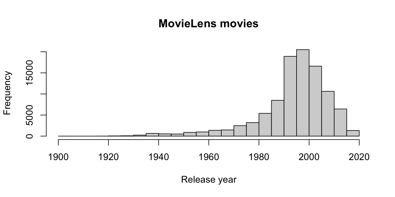
Figure 6.1: Distribution of release years in the movies data set.
The histogram (in Figure 6.1) looks pretty good. Let’s create a new variable called year that contains the year of release of the movie.
movies <- mutate(movies,
  year = str_extract(title, year_pattern) %>% as.numeric()
)
summary(movies$year)
## Min. 1st Qu. Median Mean 3rd Qu. Max. NA's
## 1902 1990 1997 1994 2003 2018 30Whoops! We have 30 NA years. Let’s take a look and see what happened.
movies %>%
  filter(is.na(year)) %>%
  select(title)
## # A tibble: 30 × 1
## title
## <chr>
## 1 "Black Mirror"
## 2 "Runaway Brain (1995) "
## 3 "The Adventures of Sherlock Holmes and Doctor Watson"
## 4 "Maria Bamford: Old Baby"
## 5 "Generation Iron 2"
## 6 "Ready Player One"
## 7 "Babylon 5"
## 8 "Ready Player One"
## 9 "Nocturnal Animals"
## 10 "Guilty of Romance (Koi no tsumi) (2011) "
## # ℹ 20 more rowsAha! Some of the movies don’t have years, so those will have to remain NA. A few other movies have an extra space after the end parentheses. We can handle the extra space with \\s*, which matches zero or more spaces.
year_pattern <- "[0-9]{4}(?=\\)\\s*$)"
movies <- mutate(movies,
  year = str_extract(title, year_pattern) %>% as.numeric()
)
summary(movies$year)
## Min. 1st Qu. Median Mean 3rd Qu. Max. NA's
## 1902 1990 1997 1994 2003 2018 17Finally, what were the five highest rated movies of 1999 that had at least 50 ratings?
movies %>%
  filter(year == 1999) %>%
  group_by(title) %>%
  summarize(mean = mean(rating), count = n()) %>%
  filter(count >= 50) %>%
  slice_max(mean, n = 5)
## # A tibble: 5 × 3
## title mean count
## <chr> <dbl> <int>
## 1 Fight Club (1999) 4.27 218
## 2 Matrix, The (1999) 4.19 278
## 3 Green Mile, The (1999) 4.15 111
## 4 Office Space (1999) 4.09 94
## 5 American Beauty (1999) 4.06 204One final common usage of regular expressions is within select. If your data frame has a lot of variables, and you want to select out some that follow a certain pattern, then knowing regular expressions can be very helpful.
Consider the accelerometer data in the fosdata package. This data set will be described in more detail in Chapter 11.
Here we list the names of all the variables in this data set:
accelerometer <- fosdata::accelerometer
names(accelerometer)
## [1] "participant"
## [2] "machine"
## [3] "set"
## [4] "contraction_mode"
## [5] "time_video_rater_cv_ms"
## [6] "time_video_rater_dg_ms"
## [7] "time_smartphone_1_ms"
## [8] "time_smartphone_2_ms"
## [9] "video_rater_mean_ms"
## [10] "smartphones_mean_ms"
## [11] "relative_difference"
## [12] "difference_video_smartphone_ms"
## [13] "mean_video_smartphone_ms"
## [14] "contraction_mode_levels"
## [15] "difference_video_raters_ms"
## [16] "difference_smartphones_ms"
## [17] "video_smartphone_difference_outlier"
## [18] "rater_difference_outlier"
## [19] "smartphone_difference_outlier"
## [20] "normalized_error_smartphone"
## [21] "participant_age_levels"
## [22] "participant_age_years"
## [23] "participant_height_cm"
## [24] "participant_weight_kg"
## [25] "participant_gender"Look at all of those variables!
Most of the data sets that we see in this book have been condensed, but it is not at all uncommon for experimenters to collect data on dozens or even hundreds of values.
Let’s suppose you wanted to create a new data frame that had all of the time measurements in it.
Those are the variables whose names end with ms.
We can do this by combining select with the regular expression ms$, which matches the letters ms and the end of the string.
select(accelerometer, matches("ms$")) %>%
  print(n = 5)
## # A tibble: 12,245 × 10
## time_video_rater_cv_ms time_video_rater_dg_ms time_smartphone_1_ms
## <dbl> <dbl> <dbl>
## 1 1340 1360 1650
## 2 1160 1180 1350
## 3 1220 1240 1400
## 4 1260 1280 1400
## 5 1560 1180 1350
## # ℹ 12,240 more rows
## # ℹ 7 more variables: time_smartphone_2_ms <dbl>,
## # video_rater_mean_ms <dbl>, smartphones_mean_ms <dbl>,
## # difference_video_smartphone_ms <dbl>,
## # mean_video_smartphone_ms <dbl>, difference_video_raters_ms <dbl>,
## # difference_smartphones_ms <dbl>To build a data frame that includes both variables that start with smartphone or end with ms, use the regular expression | character for “or.”
select(accelerometer, matches("^smartphone|ms$")) %>%
  print(n = 5)
## # A tibble: 12,245 × 11
## time_video_rater_cv_ms time_video_rater_dg_ms time_smartphone_1_ms
## <dbl> <dbl> <dbl>
## 1 1340 1360 1650
## 2 1160 1180 1350
## 3 1220 1240 1400
## 4 1260 1280 1400
## 5 1560 1180 1350
## # ℹ 12,240 more rows
## # ℹ 8 more variables: time_smartphone_2_ms <dbl>,
## # video_rater_mean_ms <dbl>, smartphones_mean_ms <dbl>,
## # difference_video_smartphone_ms <dbl>,
## # mean_video_smartphone_ms <dbl>, difference_video_raters_ms <dbl>,
## # difference_smartphones_ms <dbl>,
## # smartphone_difference_outlier <lgl>6.6 Structure of data
6.6.1 Tidy data: pivoting
The tidyverse is designed for tidy data, and a key feature of tidy data is that all data should be stored in a rectangular array, with
each row an observation and each column a variable. In particular, no information should be stored in variable names. As an example, consider the
built-in data set WorldPhones which gives the number of telephones in each region of the world, back in the day when telephones were still gaining popularity as a device for making phone calls.
The WorldPhones data is stored as a matrix with row names, so we convert it to a tibble called phones and preserve the row names in a new variable called Year. We also clean up the names into a standard format using janitor::clean_names.
phones <- as_tibble(WorldPhones, rownames = "year") %>%
  janitor::clean_names()
phones
## # A tibble: 7 × 8
## year n_amer europe asia s_amer oceania africa mid_amer
## <chr> <dbl> <dbl> <dbl> <dbl> <dbl> <dbl> <dbl>
## 1 1951 45939 21574 2876 1815 1646 89 555
## 2 1956 60423 29990 4708 2568 2366 1411 733
## 3 1957 64721 32510 5230 2695 2526 1546 773
## 4 1958 68484 35218 6662 2845 2691 1663 836
## 5 1959 71799 37598 6856 3000 2868 1769 911
## 6 1960 76036 40341 8220 3145 3054 1905 1008
## 7 1961 79831 43173 9053 3338 3224 2005 1076Notice that the column names are regions of the world, so that there is useful information stored in those names.
Every entry in this data set gives the value for a year and a region, so the tidy format should instead have three variables: year, region, and telephones. Making this change will cause this data set to become much longer. Instead of 7 rows and 7 columns, we will have 49 rows, one for each of the \(7\times7\) year and region combinations.
The tool to make this change is the pivot_longer function from the tidyr package (part of the tidyverse):
library(tidyr)phones %>%
pivot_longer(cols = !year, names_to = "region", values_to = "telephones")## # A tibble: 49 × 3
## year region telephones
## <chr> <chr> <dbl>
## 1 1951 n_amer 45939
## 2 1951 europe 21574
## 3 1951 asia 2876
## 4 1951 s_amer 1815
## 5 1951 oceania 1646
## 6 1951 africa 89
## 7 1951 mid_amer 555
## 8 1956 n_amer 60423
## 9 1956 europe 29990
## 10 1956 asia 4708
## # ℹ 39 more rowsThis function used four arguments. The first was the data frame we wanted to pivot, in this case phones. Second, we specified which columns to use, with the expression cols = !year, which meant “all columns except year.” Finally, we told the function that the names of the columns should become a new variable called “region,” and the values in those columns should become a new variable called “telephones.”
As a more complex example, let’s look at the billboard data set provided with the tidyr package.
This contains the weekly Billboard rankings for each song that entered the Top 100 during the year 2000.
Observe that each row is a song (track) and the track’s place on the charts is stored in up to 76 columns named wk1 through wk76. There are many NA in the data since none of these tracks were ranked for 76 consecutive weeks.
billboard %>% head(n = 5)## # A tibble: 5 × 79
## artist track date.entered wk1 wk2 wk3 wk4 wk5 wk6 wk7
## <chr> <chr> <date> <dbl> <dbl> <dbl> <dbl> <dbl> <dbl> <dbl>
## 1 2 Pac Baby… 2000-02-26 87 82 72 77 87 94 99
## 2 2Ge+her The … 2000-09-02 91 87 92 NA NA NA NA
## 3 3 Doors … Kryp… 2000-04-08 81 70 68 67 66 57 54
## 4 3 Doors … Loser 2000-10-21 76 76 72 69 67 65 55
## 5 504 Boyz Wobb… 2000-04-15 57 34 25 17 17 31 36
## # ℹ 69 more variables: wk8 <dbl>, wk9 <dbl>, wk10 <dbl>, wk11 <dbl>,
## # wk12 <dbl>, wk13 <dbl>, wk14 <dbl>, wk15 <dbl>, wk16 <dbl>,
## # wk17 <dbl>, wk18 <dbl>, wk19 <dbl>, wk20 <dbl>, wk21 <dbl>,
## # wk22 <dbl>, wk23 <dbl>, wk24 <dbl>, wk25 <dbl>, wk26 <dbl>,
## # wk27 <dbl>, wk28 <dbl>, wk29 <dbl>, wk30 <dbl>, wk31 <dbl>,
## # wk32 <dbl>, wk33 <dbl>, wk34 <dbl>, wk35 <dbl>, wk36 <dbl>,
## # wk37 <dbl>, wk38 <dbl>, wk39 <dbl>, wk40 <dbl>, wk41 <dbl>, …This data is not tidy, since the week column names contain information.
To do any sort of analysis on this data, the week needs to be a variable.
We use pivot_longer to replace all 76 week columns with two columns, one called “week” and another called “rank”:
long.bill <- billboard %>%
  pivot_longer(
    cols = wk1:wk76,
    names_to = "week", values_to = "rank",
    values_drop_na = TRUE
  )
long.bill
## # A tibble: 5,307 × 5
## artist track date.entered week rank
## <chr> <chr> <date> <chr> <dbl>
## 1 2 Pac Baby Don't Cry (Keep... 2000-02-26 wk1 87
## 2 2 Pac Baby Don't Cry (Keep... 2000-02-26 wk2 82
## 3 2 Pac Baby Don't Cry (Keep... 2000-02-26 wk3 72
## 4 2 Pac Baby Don't Cry (Keep... 2000-02-26 wk4 77
## 5 2 Pac Baby Don't Cry (Keep... 2000-02-26 wk5 87
## 6 2 Pac Baby Don't Cry (Keep... 2000-02-26 wk6 94
## 7 2 Pac Baby Don't Cry (Keep... 2000-02-26 wk7 99
## 8 2Ge+her The Hardest Part Of ... 2000-09-02 wk1 91
## 9 2Ge+her The Hardest Part Of ... 2000-09-02 wk2 87
## 10 2Ge+her The Hardest Part Of ... 2000-09-02 wk3 92
## # ℹ 5,297 more rowsThe values_drop_na = TRUE argument removes the NA values from the rank column while pivoting.
Which 2000 song spent the most weeks on the charts? This question would have been near impossible to answer without tidying the data. Now we can group by track and count the number of times it was ranked:
long.bill %>%
  group_by(track) %>%
  summarize(weeks_on_chart = n()) %>%
  slice_max(weeks_on_chart)
## # A tibble: 1 × 2
## track weeks_on_chart
## <chr> <int>
## 1 Higher 57Higher, by Creed, entered the charts in 2000 and spent 57 weeks in the top 100 (though not consecutively!)
The tidyr package also provides a function pivot_wider which performs the opposite transformation to pivot_longer.
You will need to provide a names_from value, which contains the variable name to get the column names from, and a values_from value or values, which gives the columns to get the cell values from.
You often will also need to provide an id_cols which uniquely identifies each observation. Let’s see how to use it in an example.
Consider the babynames data set in the babynames package. This consists of all names of babies born in the USA from 1880 through 2017, together with the sex assigned to the baby, the number of babies of that sex given that name in that year, and the proportion of babies with that sex in that year that were given the name. Only names that were given to five or more babies are included.
library(babynames)
head(babynames)
## # A tibble: 6 × 5
## year sex name n prop
## <dbl> <chr> <chr> <int> <dbl>
## 1 1880 F Mary 7065 0.0724
## 2 1880 F Anna 2604 0.0267
## 3 1880 F Emma 2003 0.0205
## 4 1880 F Elizabeth 1939 0.0199
## 5 1880 F Minnie 1746 0.0179
## 6 1880 F Margaret 1578 0.0162Convert the babynames data from year 2000 into wide format, where each row is a name together with the number of male babies and female babies with that name. Note that we need to either select down to the variables of interest or we would need to provide the id columns.
babynames %>%
  filter(year == 2000) %>%
  pivot_wider(id_cols = name, names_from = sex, values_from = n)
## # A tibble: 27,512 × 3
## name F M
## <chr> <int> <int>
## 1 Emily 25953 30
## 2 Hannah 23080 25
## 3 Madison 19967 138
## 4 Ashley 17997 82
## 5 Sarah 17697 26
## 6 Alexis 17629 2714
## 7 Samantha 17266 21
## 8 Jessica 15709 27
## 9 Elizabeth 15094 22
## 10 Taylor 15078 2853
## # ℹ 27,502 more rowsNot every name had both a male and a female entry. Those are listed as NA in the data frame. If we would prefer them to be 0, we can add values_fill = 0.
Now that we have the data in a nice format, let’s determine the most common name for which the number of male babies was within 200 of the number of female babies.
babynames %>%
  filter(year == 2000) %>%
  pivot_wider(
    id_cols = name, names_from = sex,
    values_from = n, values_fill = 0
  ) %>%
  filter(M > F - 200, M < F + 200) %>%
  mutate(total_names = F + M) %>%
  slice_max(n = 5, total_names)
## # A tibble: 5 × 4
## name F M total_names
## <chr> <int> <int> <int>
## 1 Peyton 1967 2001 3968
## 2 Skyler 1284 1472 2756
## 3 Jessie 719 533 1252
## 4 Justice 477 656 1133
## 5 Sage 557 392 949We see by this criteria, Peyton was the most common gender neutral name in 2000, followed by Skyler, Jessie, Justice, and Sage.
6.6.2 Using join to merge data frames
In this section, we introduce the join family of functions, part of the dplyr package.
We will focus on the function left_join, which joins two data frames together into one.
The syntax is left_join(x, y, by = NULL), where x and y are data frames and by is a list of columns that you want to join the data frames by
(there are additional arguments that we won’t be using).
The way to remember what left_join does is that it adds the columns of y to the columns of x by matching columns with the same names.
The band_members and band_instruments data sets are both included in the dplyr package.
band_members## # A tibble: 3 × 2
## name band
## <chr> <chr>
## 1 Mick Stones
## 2 John Beatles
## 3 Paul Beatlesband_instruments## # A tibble: 3 × 2
## name plays
## <chr> <chr>
## 1 John guitar
## 2 Paul bass
## 3 Keith guitarLeft join adds instrument information to the band member data.
left_join(band_members, band_instruments)## Joining with `by = join_by(name)`## # A tibble: 3 × 3
## name band plays
## <chr> <chr> <chr>
## 1 Mick Stones <NA>
## 2 John Beatles guitar
## 3 Paul Beatles bassWhat happens if Paul learns how to play the drums as well?
new_band_instruments## # A tibble: 4 × 2
## name plays
## <chr> <chr>
## 1 John guitar
## 2 Paul bass
## 3 Keith guitar
## 4 Paul drumsleft_join(band_members, new_band_instruments)## Joining with `by = join_by(name)`## # A tibble: 4 × 3
## name band plays
## <chr> <chr> <chr>
## 1 Mick Stones <NA>
## 2 John Beatles guitar
## 3 Paul Beatles bass
## 4 Paul Beatles drumsWhen there are multiple matches to name, then left_join makes multiple rows in the new data frame.
Here is a more compelling example where we combine data from multiple sources into a single data frame.
Consider the data sets pres_election available in the fosdata package, and unemp available in the mapproj package.
These data sets give the by county level presidential election results from 2000-2016, and the population and unemployment rate of all counties in the US.
Some packages, such as mapproj, require you to use a command like data("unemp")) to access data sets.
pres_election <- fosdata::pres_election
library(mapproj)
## Loading required package: mapsdata("unemp")Suppose we want to create a new data frame that contains both the election results and the unemployment data. That is a job for left_join.
combined_data <- left_join(pres_election, unemp, by = c("FIPS" = "fips"))Because the two data frames didn’t have any column names in common, the join required by = to specify which columns to join by.
head(combined_data)## year state state_po county FIPS candidate party
## 1 2000 Alabama AL Autauga 1001 Al Gore democrat
## 2 2000 Alabama AL Autauga 1001 George W. Bush republican
## 3 2000 Alabama AL Autauga 1001 Ralph Nader green
## 4 2000 Alabama AL Autauga 1001 Other <NA>
## 5 2000 Alabama AL Baldwin 1003 Al Gore democrat
## 6 2000 Alabama AL Baldwin 1003 George W. Bush republican
## candidatevotes totalvotes pop unemp
## 1 4942 17208 23288 9.7
## 2 11993 17208 23288 9.7
## 3 160 17208 23288 9.7
## 4 113 17208 23288 9.7
## 5 13997 56480 81706 9.1
## 6 40872 56480 81706 9.1Word to the wise: when dealing with spatial data that is organized by county, it is much easier to use the FIPS code than the county name, because there are variances in capitalization and other issues that come up when trying to use county names.
As a final example, we show how the movies data for fosdata was constructed using left_join.
MovieLens distributes their movie rating information in two separate CSV files, which you may access as follows:
movies_orig <-
  read.csv("https://stat.slu.edu/~speegle/data/ml-small/movies.csv")
ratings_orig <-
  read.csv("https://stat.slu.edu/~speegle/data/ml-small/ratings.csv")
The movies_orig data contains the movie names and genres, while the ratings_orig data contains the user ID, the rating, and the timestamp.
head(movies_orig)## movieId title genres
## 1 1 Toy Story (1995) Adventure|Animation|Chi...
## 2 2 Jumanji (1995) Adventure|Children|Fantasy
## 3 3 Grumpier Old Men (1995) Comedy|Romance
## 4 4 Waiting to Exhale (1995) Comedy|Drama|Romance
## 5 5 Father of the Bride Part II (1995) Comedy
## 6 6 Heat (1995) Action|Crime|Thrillerhead(ratings_orig)## userId movieId rating timestamp
## 1 1 1 4 964982703
## 2 1 3 4 964981247
## 3 1 6 4 964982224
## 4 1 47 5 964983815
## 5 1 50 5 964982931
## 6 1 70 3 964982400We combine the two data sets using left_join to get the movies data that we used throughout the chapter.
movies <- left_join(movies_orig, ratings_orig, by = "movieId")6.7 The apply family
This book focuses on dplyr and the tidyverse for data manipulation.
However, it can be useful to know the base R tools for doing some of the same tasks.
At a minimum, it can be useful to know these tools when reading other people’s code!
The apply family consists of quite a few functions,
including apply, sapply, lapply, vapply, tapply, mapply, and even replicate!
While tapply and its variants might be the closest in spirit to how we used dplyr in this chapter, we will focus on apply and sapply.
All of the functions in the apply family are implicit loops, like replicate.
The typical usage of apply is apply(X, MARGIN, FUN). The function apply applies the function FUN to either the rows or columns of X,
depending on whether MARGIN is 1 (rows) or 2 (columns). So, the argument X is typically a matrix or data frame and MARGIN is either 1 or 2.
The argument FUN is a function, such as sum or mean, or a custom function defined by the user.
Consider the data set USJudgeRatings, which contains the ratings of US judges by lawyers on various facets.
head(USJudgeRatings)## CONT INTG DMNR DILG CFMG DECI PREP FAMI ORAL WRIT PHYS RTEN
## AARONSON,L.H. 5.7 7.9 7.7 7.3 7.1 7.4 7.1 7.1 7.1 7.0 8.3 7.8
## ALEXANDER,J.M. 6.8 8.9 8.8 8.5 7.8 8.1 8.0 8.0 7.8 7.9 8.5 8.7
## ARMENTANO,A.J. 7.2 8.1 7.8 7.8 7.5 7.6 7.5 7.5 7.3 7.4 7.9 7.8
## BERDON,R.I. 6.8 8.8 8.5 8.8 8.3 8.5 8.7 8.7 8.4 8.5 8.8 8.7
## BRACKEN,J.J. 7.3 6.4 4.3 6.5 6.0 6.2 5.7 5.7 5.1 5.3 5.5 4.8
## BURNS,E.B. 6.2 8.8 8.7 8.5 7.9 8.0 8.1 8.0 8.0 8.0 8.6 8.6Which judge had the highest mean rating? Which rating scale had the highest mean across all judges?
Using apply across rows computes the mean rating for each judge.
head(apply(USJudgeRatings, MARGIN = 1, mean))## AARONSON,L.H. ALEXANDER,J.M. ARMENTANO,A.J. BERDON,R.I.
## 7.291667 8.150000 7.616667 8.458333
## BRACKEN,J.J. BURNS,E.B.
## 5.733333 8.116667To pull the highest mean rating:
max(apply(USJudgeRatings, MARGIN = 1, mean))## [1] 8.858333which.max(apply(USJudgeRatings, MARGIN = 1, mean))## CALLAHAN,R.J.
## 7We see that judge seven, R.J. Callahan, had the highest rating of 8.858333.
Using apply across columns computes the mean rating of all of the judges in each category.
apply(USJudgeRatings, MARGIN = 2, mean)## CONT INTG DMNR DILG CFMG DECI PREP FAMI
## 7.437209 8.020930 7.516279 7.693023 7.479070 7.565116 7.467442 7.488372
## ORAL WRIT PHYS RTEN
## 7.293023 7.383721 7.934884 7.602326Judges scored highest on the “integrity” scale.
The sapply function has as its typical usage sapply(X, FUN), where X is a vector, and FUN is the function that we wish to apply to each element of X.
You may create custom functions with the function keyword.
Approximate the sd of a \(t\) random variable with 5, 10, 15, 20, 25, and 30 degrees of freedom.
To do this for 5 df, we simulate 10,000 random values of \(t\) and take the standard deviation:
sd(rt(10000, df = 5))## [1] 1.328793To repeat this computation for the other degrees of freedom, we turn the simulation into a function we choose to call sim_t_sd.
The function takes an argument we call n and runs the simulation. In a function, the last value before the closing } is the
returned value of the function.
sim_t_sd <- function(n) {
  sd(rt(10000, df = n))
}
sim_t_sd(5) # check it for n=5
## [1] 1.260566We create a sequence of values \(5, 10, \dotsc, 30\) and then use sapply to feed each of these values to the sim_t_sd function.
sapply(X = seq(5, 30, 5), FUN = sim_t_sd)## [1] 1.292638 1.117897 1.071840 1.050075 1.047600 1.033202sapply took each element of the vector X, applied the sim_t_sd function to it, and returned the results as a vector.
Unfortunately, sapply is not type consistent in the way it simplifies results, sometimes returning a vector, sometimes a matrix.
This gives sapply a bad reputation, but it is still useful for exploratory analysis.
The function replicate is a “convenience wrapper” for a common usage of sapply, so that replicate(100, {expr}) is equivalent to sapply(1:100, function(x) {expr}), where in this case, the function inside of sapply will have no dependence on x.
Vignette: dplyr murder mystery
There has been a murder in dplyr City! You have lost your notes, but you remember that the murder took place on January 15, 2018.
All of the clues that you will need to solve the murder are contained in the dplyrmurdermystery package once you load it into your environment.
The dplyr murder mystery is a whodunit, where you use your dplyr skillz to analyze data sets that lead to the solution of a murder mystery. The original caper of this sort was the Command Line Murder Mystery,31 which was recast as SQL Murder Mystery.32
We have created an R package containing a mystery that is not entirely unlike the SQL Murder Mystery for you to enjoy. You can download the package via
remotes::install_github(repo = "speegled/dplyrmurdermystery")Once you install the package, you can load the data into your environment by typing
library(dplyrmurdermystery)
data("dplyr_murder_mystery")
This loads quite a bit of data into your environment, so you may want to make sure you are starting with a clean environment before you do it.
Vignette: Data and gender
In most studies with human subjects, the investigators collect demographic information on their subjects to control for lurking variables that may interact with the variables under investigation. One of the most commonly collected demographic variables is gender. In this vignette, we discuss current best practices for collecting gender information in surveys and studies.
Why not male or female?
The term transgender refers to people whose gender expression defies social expectations. More narrowly, the term transgender refers to people whose gender identity or gender expression differs from expectations associated with the sex assigned at birth.33
Approximately 1 in 250 adults in the US identify as transgender, with that proportion expected to rise as survey questions improve and stigma decreases.34 For teenagers, this proportion may be as high as 0.7%.35
The traditional “Male or Female?” survey question fails to measure the substantial transgender population, and the under- or non-representation of transgender individuals is a barrier to understanding social determinants and health disparities faced by this population.
How to collect gender information
Best practices36 in collecting gender information are to use a two-step approach, with the following questions:
- Assigned sex at birth: What sex were you assigned at birth, on your original birth certificate?
- Male
- Female
- Current gender identity: How do you describe yourself? (check one)
- Male
- Female
- Transgender
- Do not identify as female, male, or transgender
These questions serve as guides. Question 1 has broad agreement, while there is still discussion and research being done as to what the exact wording of Question 2 should be. It is also important to talk to people who have expertise in or familiarity with the specific population you wish to sample from, to see whether there are any adjustments to terminology or questions that should be made for that population.
In general, questions related to sex and gender are considered “sensitive.” Respondents may be reluctant to answer sensitive questions or may answer inaccurately. For these questions, privacy matters. When possible, place sensitive questions on a self-administered survey. Placing gender and sexual orientation questions at the start of a survey may also decrease privacy, since those first questions are encountered at the same time for all subjects and are more visible on paper forms.
How to incorporate gender in data analysis
The relatively small samples of transgender populations create challenges for analysis. One type of error is called a specificity error and occurs when subjects mistakenly indicate themselves as transgender or another gender minority. The transgender population is less than 1% of the overall population. So, if even one in one hundred subjects misclassifies themselves, then the subjects identifying as transgender in the sample will be a mix of half transgender individuals and half misclassified individuals. The best way to combat specificity errors is with carefully worded questions and prepared language to explain the options if asked.
Small samples lead to a large margin of error and make it difficult to detect statistically significant differences within groups.37 For an individual survey, this may prevent analysis of fine-grained gender information. Aggregating data over time, space, and across surveys can allow analysis of gender minority groups.
Example
The data fosdata::gender was collected by Sell, Goldberg, and Conron38 to determine if it is feasible to sample from rare and dispersed populations using the online service “Google Android Panel.”
They use the two-step approach to gender, with a sex-at-birth question and a gender identity question that is broadly worded and that allows respondents
to select multiple options. This multiple-option question is coded as seven different T/F variables beginning with gender_.
gender <- fosdata::gender
str(gender)
## 'data.frame': 20305 obs. of 10 variables:
## $ gender_male : logi FALSE FALSE FALSE FALSE FALSE TRUE ...
## $ gender_female : logi TRUE TRUE TRUE TRUE TRUE FALSE ...
## $ gender_trans : logi FALSE FALSE FALSE TRUE FALSE FALSE ...
## $ gender_queer : logi FALSE FALSE FALSE FALSE FALSE FALSE ...
## $ gender_not_sure: logi FALSE FALSE FALSE FALSE FALSE FALSE ...
## $ gender_unclear : logi FALSE FALSE FALSE FALSE FALSE FALSE ...
## $ gender_na : logi FALSE FALSE FALSE FALSE FALSE FALSE ...
## $ sex_at_birth : Factor w/ 2 levels "Female","Male": 1 1 1 1 1 2 1 ..
## $ hispanic : Factor w/ 3 levels "Don't know","No",..: 2 2 2 2 2..
## $ race : chr "White" "White" "Black or African American" "..As a first step, let’s explore how many respondents selected more than one option:
gender <- gender %>%
  mutate(responses = rowSums(across(matches("^gender"))))
table(gender$responses)
##
## 1 2 3 4 5 6
## 20050 200 34 1 3 17Here we used dplyr’s across function to say we want to take row sums of responses across all variables that start with “gender.” When summing,
TRUE values count as 1.
Observe that the vast majority of the respondents selected only one value. However, the prevalence of respondents with two or more values is not small when compared with the number of non-cisgender individuals (only 757 as we will see shortly). In particular, 17 individuals answered yes to six of the seven gender questions available, and those answers seem likely to be due to user confusion or error possibly leading to specificity error in our results.
Following Sell et al., we compute a “transgender status” summary variable which labels respondents reporting:
- current gender identity of male and being assigned male at birth as “Male (cisgender)”
- current gender identity of female and being assigned female at birth as “Female (cisgender)”
- current gender identity of male, transgender, or genderqueer/gender non-conforming and being assigned female at birth as “Male,Trans,GenQ/Female@Birth”
- current gender identity of female, transgender, or genderqueer/gender non-conforming and being assigned male at birth as “Female,Trans,GenQ/Male@Birth”
We use dplyr’s case_when statement to select the cases.
gender <- gender %>%
  mutate(trans_status = case_when(
    sex_at_birth == "Male" & gender_male & responses == 1 ~
      "Male (cisgender)",
    sex_at_birth == "Female" & gender_female & responses == 1 ~
      "Female (cisgender)",
    sex_at_birth == "Female" & gender_male | gender_trans | gender_queer ~
      "Male,Trans,GenQ/Female@Birth",
    sex_at_birth == "Male" & gender_female | gender_trans | gender_queer ~
      "Female,Trans,GenQ/Male@Birth"
  ))
gender %>%
  group_by(trans_status) %>%
  summarize(n())
## # A tibble: 5 × 2
## trans_status `n()`
## <chr> <int>
## 1 Female (cisgender) 9733
## 2 Female,Trans,GenQ/Male@Birth 47
## 3 Male (cisgender) 9815
## 4 Male,Trans,GenQ/Female@Birth 396
## 5 <NA> 314We finish this example by making a table of trans status gender by race. For simplicity, we only look at respondents with a single answer to the race question and ignore the hispanic variable.
gender %>%
  filter(!stringr::str_detect(race, ",")) %>%
  mutate(trans = stringr::str_detect(trans_status, "Trans")) %>%
  group_by(race) %>%
  summarize(
    respondents = n(),
    trans_pct = round(100 * mean(trans, na.rm = TRUE), 1)
  )
## # A tibble: 6 × 3
## race respondents trans_pct
## <chr> <int> <dbl>
## 1 American Indian or Alaskan Native 170 9.1
## 2 Asian 1647 1.5
## 3 Black or African American 1212 2.1
## 4 None of the above 626 3.2
## 5 Some other race 842 3.6
## 6 White 13443 1.5Exercises
Exercises 6.1 – 6.2 require material through Section 6.2.
The built-in data set iris is a data frame containing measurements of the sepals and petals of 150 iris flowers. Convert this data to a tibble
with new variables Sepal.Area and Petal.Area which are the product of the corresponding length and width measurements.
Consider the austen data set in the fosdata package.
This data frame contains the complete texts of Emma and Pride and Prejudice, with additional information which you can read about in the help page for the data set. Each of the following tasks corresponds to using a single dplyr verb.
- Create a new data frame that consists only of the observations in Emma.
- Create a new data frame that contains only the variables
word,word_lengthandnovel. - Create a new data frame that has the words in both books arranged in descending word length.
- Create a new data frame that contains only the longest words that appeared in either of the books.
- What was the mean word length in the two books together?
- Create a new data frame that consists only of the distinct words found in the two books, together with the word length and sentiment score variables. (Hint: use
distinct).
Exercises 6.3 – 6.26 require material through Section 6.4.
Consider the mpg data set in the ggplot2 package. For the purposes of this question, consider each observation a different car.
- Which car(s) had the highest highway gas mileage?
- Compute the mean city mileage for compact cars.
- Compute the mean city mileage for each class of cars, and arrange in decreasing order.
- Which cars have the smallest absolute difference between highway mileage and city mileage?
- Compute the mean highway mileage for each year, and arrange in decreasing order.
This question uses the DrinksWages from the HistData package.
This data, gathered in 1910, was a survey of people working in various trades (bakers, plumbers, goldbeaters, etc.).
The trades are assigned class values of A, B, or C based on required skill.
For each trade, the number of workers who drink (drinks), the number of sober workers (sober), and wage information (wage) was recorded.
There is also a column n = drinks + sober which is the total number of workers surveyed for each trade.
- Compute the mean wages for each class, A, B, and C.
- Find the three trades with the highest proportion of drinkers. Consider only trades with 10 or more workers in the survey.
Consider the data set oly12 from the VGAMdata package (that you will probably need to install).
It has individual competitor information from the Summer 2012 London Olympic Games.
- According to this data, which country won the most medals? How many did that country win? (You need to sum Gold, Silver, and Bronze.)
- Which countries were the heaviest? Compute the mean weight of male athletes for all countries with at least 10 competitors, and report the top three.
Exercises 6.6 – 6.10 all use the movies data set from the fosdata package.
What is the movie with the highest mean rating that has been rated at least 30 times?
Which genre has been rated the most? (For the purpose of this, consider Comedy and Comedy|Romance as completely different genres, for example.)
Which movie in the genre Comedy|Romance that has been rated at least 50 times has the lowest mean rating? Which has the highest mean rating?
Which movie that has a mean rating of 4 or higher has been rated the most times?
Which user gave the highest mean ratings?
Exercises 6.11 – 6.16 all use the Batting data set from the Lahman package.
This gives the batting statistics of every player who has played baseball from 1871 through the present day.
Which player has been hit-by-pitch the most number of times?
How many doubles were hit in 1871?
Which team has the most total number of home runs, all time?
Which player who has played in at least 500 games has scored the most number of runs per game?
- Which player has the most lifetime at bats without ever having hit a home run?
- Which active player has the most lifetime at bats without ever having hit a home run? (An active player is someone with an entry in the most recent year of the data set).
- Verify that Curtis Granderson hit the most triples in a single season since 1960.
- In which season did the major league leader in triples have the fewest triples?
- In which season was there the biggest difference between the major league leader in stolen bases (SB) and the player with the second most stolen bases?
Exercises 6.17 – 6.24 all use the Pitching data set from the Lahman package.
This gives the pitching statistics of every pitcher who has played baseball from 1871 through the present day.
- Which pitcher has won (W) the most number of games?
- Which pitcher has lost (L) the most number of games?
Which pitcher has hit the most opponents with a pitch (HBP)?
Which year had the most number of complete games (CG)?
Among pitchers who have won at least 100 games, which has the highest winning percentage? (Winning percentage is wins divided by wins + losses.)
Among pitchers who have struck out at least 500 batters, which has the highest strikeout to walk ratio? (Strikeout to walk ratio is SO/BB.)
List the pitchers for the St Louis Cardinals (SLN) in 2006 with at least 30 recorded outs (IPouts), sorted by ERA from lowest to highest.
A balk (BK) is a subtle technical mistake that a pitcher can make when throwing. What were the top five years with the most balks in major league baseball history? Why was 1988 known as “the year of the balk”?
Which pitcher has the most outs pitched (IPouts) of all the pitchers who have more bases on balls (BB) than hits allowed (H)? Who has the second-most?
Consider the storms data set in the dplyr package, from Example 6.5. Recall that name and year together identify all storms except Zeta (2005-2006).
- Which name(s) was/were given to the most storms?
- Which year(s) had the most named storms?
- The second strongest storm named Lili had maximum wind speed of 100. Which name’s second strongest storm in terms of maximum wind speed was the strongest among all names’ second strongest storms? The
dplyrfunctionnthmay be useful for doing this problem.
M&M’s are small pieces of candy that come in various colors and are sold in various sizes of bags. One popular size for Halloween is the “Fun Size,” which typically contains between 15 and 18 M&M’s. For the purposes of this problem, we assume the mean number of candies in a bag is 17 and the standard deviation is 1. According to Rick Wicklin39, the proportion of M&M’s of various colors produced in the New Jersey M&M factory are as follows.
| Color | Proportion |
|---|---|
| Blue | 25.0 |
| Orange | 25.0 |
| Green | 12.5 |
| Yellow | 12.5 |
| Red | 12.5 |
| Brown | 12.5 |
Suppose that you purchase a big bag containing 200 Fun Size M&M packages. The purpose of this exercise it to estimate the probability that each of your bags has a different distribution of colors.
- We will model the number of M&M’s in a bag with a binomial random variable. Find values of \(n\) and \(p\) such that a binomial random variable with parameters \(n\) and \(p\) has mean approximately 17 and variance approximately 1.
- (Hard) Create a data frame that has its rows being bags and columns being colors, where each entry is the number of M&M’s in that bag of that color. For example, the first entry in the first column might be 2, the number of Blue M&M’s in the first bag.
- Use
nrowsanddplyr::distinctto determine whether each row in the data frame that you created is distinct. - Put inside
replicateand estimate the probability that all bags will be distinct. This could take some time to run, depending on how you did parts (b) and (c), so start with 500 replicates.
Exercises 6.27 – 6.33 require material through Section 6.5.
The data set words is built into the stringr package.
- How many words in this data set contain “ff”?
- What percentage of these words start with “s”?
The data set sentences is built into the stringr package.
- What percentage of sentences contain the string “the”?
- What percentage of sentences contain the word “the” (so, either “the” or “The”)?
- What percentage of sentences start with the word “The”?
- Find the one sentence that has both an “x” and a “q” in it.
- Which words are the most common words that a sentence ends with?
The data set fruit is built into the stringr package.
- How many fruits have the word “berry” in their name?
- Some of these fruits have the word “fruit” in their name. Find these fruit and remove the word “fruit” to create a list of words that can be made into fruit. (Hint: use
str_remove)
Exercises 6.30 – 6.32 require the babynames data frame from the babynames package.
Say that a name is popular if it was given to 1000 or more babies of a single sex. How many popular female names were there in 2015? What percentage of these popular female names ended in the letter ‘a’?
Consider the babynames data set. Restrict to babies born in 2003. We’ll consider a name to be gender neutral if the number of male babies given that name is within plus or minus 20% of the number of girl babies given that name. What were the 5 most popular gender neutral names in 2003?
The phonics package has a function metaphone that gives a rough phonetic transcription of English words.
Restrict to babies born in 2003 and create a new variable called phonetic, which gives the phonetic transcription of the names.
- Filter the data set so that the year is 2003 and so that each phonetic transcription has at least two distinct names associated with it.
- Filter the data so that it only contains the top 2 most given names for each phonetic transcription.
- Among the pairs of names for girls obtained in the previous part with the same metaphone representation and such that each name occurs less than 120% of the times that the other name occurs, which pair of names was given most frequently?
- We wouldn’t consider the most common pair to actually be the “same name.” Look through the list sorted by total number of times the pair of names occurs, and state which pair of names that you would consider to be the same name is the most common. That pair is, in some sense, the hardest to spell common name from 2003.
- What is the most common hard to spell triple of girls names from 2003? (Answers may vary, depending on how you interpret this. To get interesting answers, you may need to loosen the 120% rule from the previous part.)
In this exercise, we examine the expected number of coin tosses until various patterns occur.
For each pattern given below, find the expected number of tosses until the pattern occurs.
For example, if the pattern is HTH and you toss HHTTHTTHTH, then it would be 10 tosses until HTH occurs.
With the same sequence of tosses, it would be 5 tosses until TTH occurs.
(Hint: paste(coins, collapse = "") converts a vector containing H and T into a character string on which you can use stringr commands such as str_locate.)
- What is the expected number of tosses until HTH occurs?
- Until HHT occurs?
- Until TTTT occurs?
- Until THHH occurs?
Exercises 6.34 – 6.37 require material through Section 6.6.
This exercise uses the billboard data from the tidyr package.
- Which artist had the most tracks on the charts in 2000?
- Which track from 2000 spent the most weeks at #1? (This requires tidying the data as described in Section 6.6.1.)
Consider the scrabble and letter_frequency data sets in the fosdata package.
- Create a new data frame that contains the variables
letter,points,number, andfrequencyfor all English letters a through z.numbershould be the number of tiles in a Scrabble set with that letter, andfrequencyshould be the letter frequency fromletter_frequency - Which letter has the largest absolute difference between the percentage of tiles that are that letter and the frequency of that letter occurring in
letter_frequency? Note that the frequency of tiles in Scrabble should be related to the frequency of letters in the dictionary. The data setletter_frequencygives the frequency in texts, so we would not expect the frequencies to match.
Consider the scotland_births data set in the fosdata package.
This data gives the number of births by the age of the mother in Scotland for each year from 1945-2019. This data is in wide format. (Completion of this exercise will be helpful for Exercise 7.28.)
- Convert the data into long format with three variable names:
age,yearandbirths, where each observation is the number ofbirthsinyearto mothers that areageyears old. - Convert the year to integer by removing the
xand usingas.integer. - Which year had the most babies born to mothers 20-years-old or younger?
The data set world_cup from fosdata has the results of all games in the 2014 and 2015 FIFA World Cup soccer finals.
From this data, create a data frame which has the total number of goals scored by each team in the 2015 World Cup. Your data frame
should have only two variables, team and goals, and 24 rows, one for each team. Display the entire data frame in descending order of goals scored.
Exercise 6.38 requires material through Section 6.7.
Suppose you sample five numbers from a uniform distribution on the interval \([0, 1]\). Use simulation to show that the expected value of the \(k\)th smallest of the five values is \(\frac{k}{6}\). That is, the minimum of the five values has expected value 1/6, the second smallest of the values has expected value 2/6, and so on.
Loading
dplyrproduces warning messages because thedplyrpackage contains commands that override some base R commands (notably thefiltercommand). This book will not show these warnings. UsesuppressMessages(library(dplyr))if you want to load the package quietly.↩︎F Maxwell Harper and Joseph A Konstan, “The MovieLens Datasets: History and Context,” ACM Trans. Interact. Intell. Syst. 5, no. 4 (December 2015), https://doi.org/10.1145/2827872.↩︎
If filter reports an error such as
Error in filter(movies, rating <= 1) : object 'rating' not foundthat you don’t understand, it is likely that you forgot to load thedplyrpackage. Load it withlibrary(dplyr).↩︎Rating should almost certainly have been reclassified as an ordered factor, and it is not clear that taking the mean is really a valid thing to do.↩︎
This is a lie. There was one storm, Zeta, which formed on December 30, 2005 and lasted until January 6, 2006. It and the unusual storm Eta, also from 2005, are the subject of an XKCD comic, https://xkcd.com/1126/.↩︎
If you definitely want to see all of the movies, you can pipe to
print(n = nrow(.))↩︎Marla Berg-Weger, Social Work and Social Welfare: An Invitation (Routledge, 2016).↩︎
Esther L Meerwijk and Jae M Sevelius, “Transgender Population Size in the United States: A Meta-Regression of Population-Based Probability Samples,” American Journal of Public Health 107, no. 2 (2017): e1–8, https://doi.org/10.2105/AJPH.2016.303578.↩︎
N Chokshi, “One in Every 137 Teenagers Would Identify as Transgender, Report Says,” The New York Times, February 23, 2017.↩︎
The GenIUSS Group, “Best Practices for Asking Questions to Identify Transgender and Other Gender Minority Respondents on Population-Based Surveys,” ed. J. L. Herman (Los Angeles, CA: The Williams Institute, 2014).↩︎
These terms are defined in Chapter 8. If these terms are new to you, just think of it for now as meaning that it is hard to get information from small amounts of data.↩︎
Randall Sell, Shoshana Goldberg, and Kerith Conron, “The Utility of an Online Convenience Panel for Reaching Rare and Dispersed Populations,” PLOS One 10 (December 2015): e0144011, https://doi.org/10.1371/journal.pone.0144011.↩︎
Purtill, “A Statistician Got Curious about M&M Colors and Went on an Endearingly Geeky Quest for Answers.”↩︎