Chapter 12 Analysis of Variance and Comparison of Multiple Groups
In this chapter, we introduce one-way analysis of variance (ANOVA) through the analysis of a motivating example.
Viñals et al.109 studied the effects of marijuana on mice. One group of ordinary (“wild type”) mice were given a dose of tetrahydrocannabinol (THC), the active ingredient in marijuana. Another group of wild type mice were given a vehicle, which is a shot with the same inactive ingredients but no THC.
George Shuklin. This file is licensed under the Creative Commons Attribution-Share Alike 1.0 Generic license. https://commons.wikimedia.org/wiki/File:Мышь_2.jpg
The investigators measured the locomotor activity of the mice by placing each mouse in a box lined with photocells and then observing the total distance traveled by the mouse. The results were reported as the percentage movement relative to the untreated VEH group, so values over 100 represent mice that moved a lot, and values under 100 represent mice that moved less.
Data from the mouse study is in the fosdata package in the mice_pot data set.
mice_pot <- fosdata::mice_potThe data consists of 42 observations of 2 variables.
The variable group is the dosage of THC that each mouse received,
and percent_of_act measures locomotion as the percent of baseline activity.
Start by exploring the data with summary statistics in Table 12.1 and a boxplot.
mice_pot %>%
  group_by(group) %>%
  summarize(
    mean = mean(percent_of_act),
    sd = sd(percent_of_act),
    skew = e1071::skewness(percent_of_act),
    N = n()
)| group | mean | sd | skew | N |
|---|---|---|---|---|
| VEH | 100.000 | 25.324 | -0.190 | 15 |
| 0.3 | 97.323 | 31.457 | 0.133 | 9 |
| 1 | 99.052 | 26.258 | -0.106 | 12 |
| 3 | 70.668 | 20.723 | 0.034 | 10 |
ggplot(mice_pot, aes(x = group, y = percent_of_act)) +
  geom_boxplot(outlier.size = -1) +
  geom_jitter(height = 0, width = .2)
The plot and summary statistics show that there is little difference between the first three groups, but once the dose gets up to 3 mg/kg, the mice appear to be moving less.
This chapter introduces a number of different hypothesis tests to test for a difference in the means of multiple groups. The first we consider is one-way analysis of variance, abbreviated ANOVA.
For the mice, one-way ANOVA will test whether the amount of movement is the same in all four groups. ANOVA requires values in each group to be normally distributed, equal variance across groups, and independence. From the boxplot, mouse locomotion appears to be normally distributed, and each group has approximately the same variance. We know from the experimental design that the measurements on each mouse are independent.
To run one-way ANOVA on the mouse experiment, first build a linear model of percent_of_act as explained by group,
then run the anova command on the linear model:
mice_model <- lm(percent_of_act ~ group, data = mice_pot)
anova(mice_model)
## Analysis of Variance Table
##
## Response: percent_of_act
## Df Sum Sq Mean Sq F value Pr(>F)
## group 3 6329 2109.65 3.1261 0.0357 *
## Residuals 42 28344 674.85
## ---
## Signif. codes: 0 '***' 0.001 '**' 0.01 '*' 0.05 '.' 0.1 ' ' 1The next section will explain the complex output of the anova function fully. The \(p\)-value for the test is given by the Pr(>F) field,
so \(p = 0.0357\) for this data, and the * means significance at the \(\alpha = 0.05\) level.
We reject the hypothesis that the mean percent of activity is the same for all four groups. The association between THC treatment and locomotion is unlikely to be due to chance.
12.1 ANOVA
One-way ANOVA is used when a single quantitative variable \(Y\) is measured on multiple groups. We will only be interested in the case where there is one categorical variable (the grouping) to explain \(Y\).
12.1.1 Groups and means
One-way ANOVA involves multiple observations over multiple groups, so the notation required is fairly complex:
- There are \(N\) total observations.
- There are \(k\) groups.
- There are \(n_i\) observations in the \(i\)th group.
- \(y_{ij}\) denotes the \(j\)th observation from the \(i\)th group.
- \(\overline{y}_{i\cdot}\) denotes the mean of the observations in the \(i\)th group.
- \(\overline{y}_{\cdot}\) denotes the mean of all observations.
In mice_pot there are 4 groups so \(k=4\).
The observed variable \(Y\) is percent_of_act, percent of activity relative to baseline.
From the following table, we see that \(n_1 = 15\), \(n_2 = 9\), \(n_3 = 12\), and \(n_4 = 10\).
table(mice_pot$group)##
## VEH 0.3 1 3
## 15 9 12 10There are 46 observations, so \(N = 46\).
In group 1, the VEH group, we have \(y_{11} = 54.2\), \(y_{12} = 65.9\), and so on. This means the first mouse in group 1 has activity 54.2% of baseline, and the second had 65.9%. In group 2, the first mouse has activity \(y_{21} = 98.8\), and in group three the first mouse has activity \(y_{31} = 95.3\).
To compute the group means:
mice_pot %>%
  group_by(group) %>%
  summarize(round(mean(percent_of_act), 1))
## # A tibble: 4 × 2
## group `round(mean(percent_of_act), 1)`
## <fct> <dbl>
## 1 VEH 100
## 2 0.3 97.3
## 3 1 99.1
## 4 3 70.7This tells us that \(\overline{y}_{1\cdot} = 100\) and \(\overline{y}_{4\cdot} = 70.7\). Group 1, the VEH group, is exactly 100 by definition, since the percentage of activity was based on what the VEH group did.
To get the overall mean, we use mean(mice_pot$percent_of_act), which gives \(\overline{y}_{\cdot} = 92.9\).
The first step to running an analysis of variance in R is to fit a linear model
to the data with the lm command.
The syntax is the same as when running simple linear regressions, a formula of the form y ~ x, where x is
the explanatory variable, y is the response variable, and the ~ (tilde) character can be read as “explained by”.
When the explanatory variable is categorical, lm chooses one of the \(k\) groups defined by x to act as the base level,
the first group alphabetically or in the factor order.
It then introduces \(k-1\) variables taking their names from the names
of the other groups defined by x. The linear model is presented as an “intercept,” which is really the mean of the base level, and
“coefficients” which are simply the differences between the base level group mean \(\overline{y}_{1\cdot}\) and the other group means \(\overline{y}_{i\cdot}\). Chapter 13 goes into more detail.
Using mice_pot, form the linear model explaining percent of activity by treatment group.
lm(percent_of_act ~ group, data = mice_pot)##
## Call:
## lm(formula = percent_of_act ~ group, data = mice_pot)
##
## Coefficients:
## (Intercept) group0.3 group1 group3
## 100.0000 -2.6775 -0.9477 -29.3321The intercept is 100, which is the mean percent of activity in the VEH group. The other treatment means are given by adding
the appropriate coefficient to 100. For example, the mean percent of activity in the 3 mg/kg group is \(100 - 29.3321 = 70.6679\).
Because the linear model presents the data as relative to the base level, the coefficients can only compare the groups to the base level, not to each other. Since the base level is often arbitrary, we do not perform inference directly on the model. Instead, we rely on analysis of variance.
12.1.2 The ANOVA model
For one-way ANOVA, the cell means model for observations is
\[ y_{ij} = \mu_i + \epsilon_{ij}, \]
Here, \(y_{ij}\) represents the \(j^\text{th}\) observation of the \(i^\text{th}\)treatment. The parameters \(\mu_i\) represent the means of the treatment groups and will be estimated from data. The values of \(\epsilon_{ij}\) account for the variation within the group. In the one-way ANOVA model, \(\epsilon_{ij}\) are independent normal random variables with mean zero and common standard deviation \(\sigma\).
Using estimates from the data each individual data point is described by \[ y_{ij} = \overline{y}_\cdot + (\overline{y}_{i\cdot} - \overline{y}_\cdot) + (y_{ij} - \overline{y}_{i\cdot}) \]
The null hypothesis for ANOVA is that the group means are all equal. That is:
- \(H_0\): \(\mu_1 = \mu_2 = \cdots =\mu_k\),
- \(H_a\): Not all \(\mu_i\) are equal.
ANOVA is “analysis of variance” because we will compare the variation of data within individual groups with the variation between groups. We make assumptions (see Assumptions 12.1) to predict the behavior of this comparison when \(H_0\) is true. If the observed behavior is extreme, then it gives evidence against the null hypothesis. The general idea of comparing variance within groups to the variance between groups is applicable in a wide variety of situations.
The sum of squares within groups110 is the sum of squares of residuals: \[ SS_R = \sum_i \sum_j (y_{ij} - \overline{y}_{i\cdot})^2. \]
The sum of squares between groups is associated with the grouping factor as: \[ SS_B = \sum_i\sum_j (\overline{y}_{i\cdot} - \overline{y})^2. \]
The sum of squares total is \[ SS_{\text{tot}} = \sum_i \sum_j (\overline{y} - y_{ij})^2. \]
The key mathematical result is the following theorem.
The total variation is the sum of the variation between groups and the variation within the groups. Using the notation in Definition 12.3,
\[ SS_{\text{tot}} = SS_R + SS_B. \]
If the variation between groups is much larger than the variation within groups, then that is evidence that there is a difference in the means of the groups. The question then becomes: how large is large? In order to answer that, we will need to examine the \(SS_B\) and \(SS_R\) terms more carefully.
- The population of each group is normally distributed.
- The variances of the groups are equal.
- The observations are independent.
Assumption 1 is typical of parametric statistics, because it provides a way to identify the data with known distributions.
Assumption 2 is a big one, and is investigated thoroughly in Section 12.3. There is no theoretical reason why the groups would have equal variances, so this must be checked.
Assumption 3 is dependent on the experimental design. A common experimental design that violates Assumption 3 is to use the same unit in each group. Suppose the THC mouse experiment used the mice repeatedly, giving each of the four treatments to each mouse. Then the independence assumption would be false and one-way ANOVA would be inappropriate. This mirrors the distinction between paired and independent two sample tests.
The test statistic for one-way ANOVA is \[ F = \frac{SS_B/(k - 1)}{SS_R/(N - k)}. \] If the Assumptions (12.1) for one-way ANOVA are met, then \(F\) has the \(F\) distribution with \(k-1\) and \(N-k\) degrees of freedom.
We have \(k\) groups. There are \(n_i\) observations in group \(i\), and \(N = \sum n_i\) total observations.
Notice that \(SS_R\) is almost \(\sum\sum (\overline{y}_{ij} - \mu_i)^2\), in which case \(SS_R/\sigma^2\) would be a \(\chi^2\) random variable with \(N\) degrees of freedom. However, we are making \(k\) replacements of means by their estimates, so we subtract \(k\) to get that \(SS_R/\sigma^2\) is \(\chi^2\) with \(N - k\) degrees of freedom. (This follows the heuristic we started in Section 10.4.)
As for \(SS_B\), it is trickier to see, but \(\sum_i \sum_j (y_{i\cdot} - \mu)^2/\sigma^2\) would be \(\chi^2\) with \(k\) degrees of freedom. Replacing \(\mu\) by \(\overline{y}\) makes \(SS_B/\sigma^2\) a \(\chi^2\) rv with \(k - 1\) degrees of freedom.
The test statistic is \[ F = \frac{SS_B/(k - 1)}{SS_R/(N - k)} = \frac{(SS_B/\sigma^2)/(k - 1))}{(SS_R/\sigma^2)/(N - k))} \]
This is the ratio of two \(\chi^2\) rvs divided by their degrees of freedom; hence, it is \(F\) with \(k - 1\) and \(N - k\) degrees of freedom.
Though this derivation lacks details, it explains why Assumptions 12.1 are necessary. The assumption of equal variances is needed to cancel the unknown \(\sigma^2\). The normality assumption is needed so that we get a known distribution for the test statistic.
12.1.3 Simulations
In this section, we confirm through simulation that the test statistic under the null hypothesis does have an \(F\) distribution.
We must assume normality and equal variances, and we wish to simulate the test statistic under the null hypothesis that all means are equal. So, we assume three populations, all of which are normally distributed with mean 0 and standard deviation 1. We arbitrarily decide to use 10 samples from group 1, 20 from group 2, and 30 from group 3, giving \(k = 3\) and \(N = 60\).
three_groups <- data.frame(
  group = rep(1:3, times = c(10, 20, 30)),
  value = rnorm(60, 0, 1)
)
We could use built-in R functions to compute the test statistic, but it is worthwhile to understand all of the formulas so we do it step by step.
We first make sure that group is a factor! We can also check that (in this case, anyway) \(SS_R + SS_B = SS_\text{tot}\).
three_groups$group <- factor(three_groups$group)
sse <- three_groups %>%
  mutate(total_mean = mean(value)) %>%
  group_by(group) %>%
  mutate(
    mu = mean(value),
    diff_within = value - mu,
    diff_between = mu - total_mean,
    diff_tot = value - total_mean
  ) %>%
  ungroup() %>%
  summarize(
    sse_within = sum(diff_within^2),
    sse_between = sum(diff_between^2),
    sse_total = sum(diff_tot^2)
  )
sse
## # A tibble: 1 × 3
## sse_within sse_between sse_total
## <dbl> <dbl> <dbl>
## 1 45.2 1.46 46.7Now that we have computed the three sums of squared errors, we verify that \(SS_R + SS_B = SS_\text{tot}\).
sse$sse_within + sse$sse_between - sse$sse_total## [1] -1.421085e-14Now we can compute the test statistic.
k <- 3
N <- 60
(sse$sse_between / (k - 1)) / (sse$sse_within / (N - k))
## [1] 0.9198313For simulation, it is faster to use the anova command to compute \(F\) directly:
aov.mod <- anova(lm(value ~ group, data = three_groups))
aov.mod$`F value`[1]
## [1] 0.9198313Now we are ready for the simulation.
sim_data <- replicate(1000, {
  three_groups <- data.frame(
    group = rep(1:3, times = c(10, 20, 30)),
    value = rnorm(60, 0, 1)
  )
  three_groups$group <- factor(three_groups$group)
  aov.mod <- anova(lm(value ~ group, data = three_groups))
  aov.mod$`F value`[1]
})
plot(density(sim_data),
  main = "F test statistic"
)
curve(df(x, 2, 57), add = T, col = 2)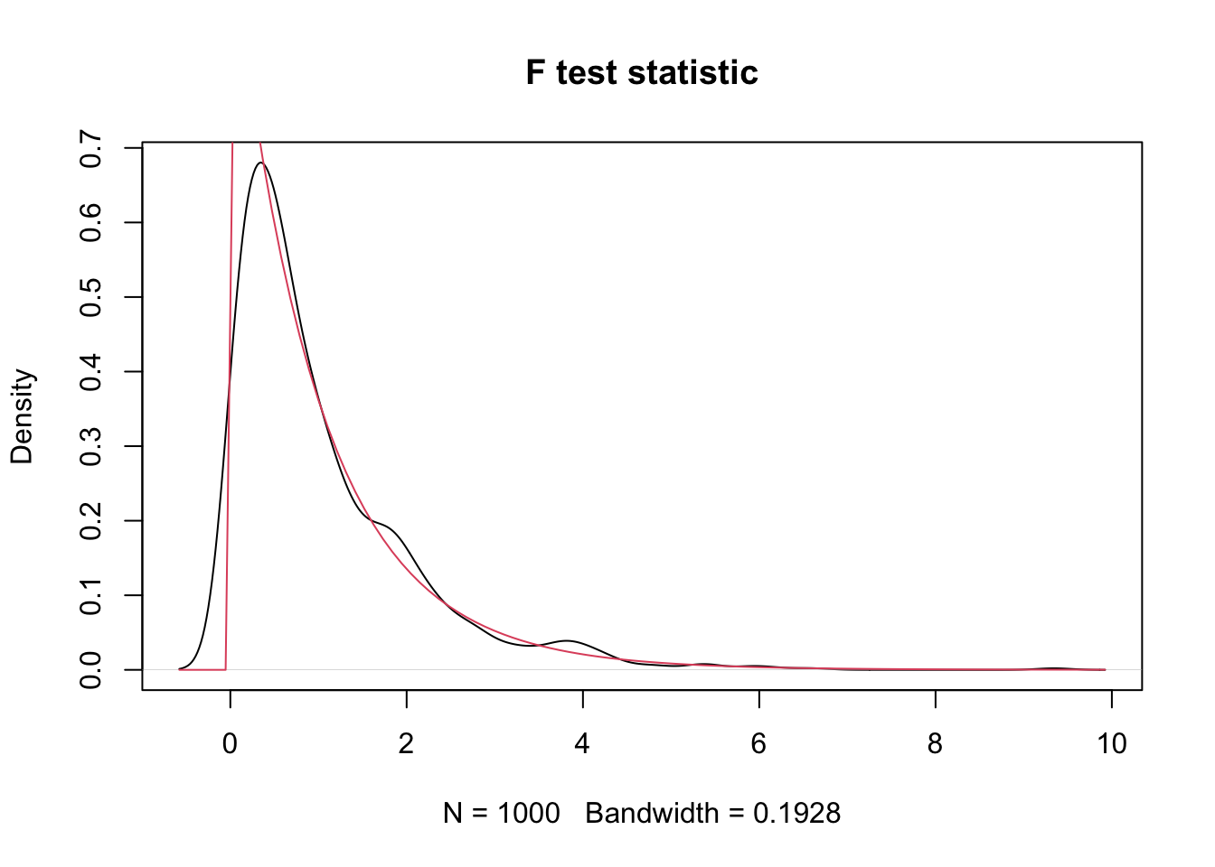
Indeed, the test statistic distribution matches the \(F\) distribution with 2 and 57 degrees of freedom.
12.2 The ANOVA test
To perform analysis of variance, compute the test statistic \(F\). Because large values of \(F\) are more likely under \(H_a\) than under \(H_0\), while small values of \(F\) are more likely under \(H_0\) than under \(H_A\), ANOVA is a one-sided test.
If \(F\) is large enough, as determined by the appropriate \(F\) distribution, then we reject \(H_0: \mu_1 = \mu_2 = \cdots =\mu_k\) in favor of the alternative hypothesis that not all of the \(\mu_i\) are equal. More precisely, the \(p\)-value is the probability of observing a value as large as \(F\) or larger from the \(F(k-1,N-k)\) distribution.
To perform ANOVA in R, use lm to build a linear model of the numeric variable on the grouping variable. Then run anova on the model object.
When performing ANOVA in R, it is essential that the grouping variable is a factor. If the grouping variable is numeric, then R will fit a line to the data, which would be inappropriate. R will not warn you about this. For this reason, always check that the degrees of freedom matches the number of groups minus 1. If degrees of freedom is 1 and you have more than two groups, then you likely miscoded the grouping variable.
12.2.1 Example: THC mice
At the start of the chapter, we used anova to analyze the differences between four groups of mice given different doses of THC.
In this section, we step through that computation carefully.
The data is in fosdata::mice_pot. We have already seen that the four distributions are approximately normal with
approximately equal variance, and the measurements are independent.
The null hypothesis is
\(H_0: \mu_1 = \mu_2 = \mu_3 = \mu_4\), where \(\mu_i\) is the true mean percent activity relative to baseline.
The alternative hypothesis is that at least one of the means is different. We will test at the \(\alpha = .05\) level.
mice_mod <- lm(percent_of_act ~ group, data = mice_pot)
anova(mice_mod)
## Analysis of Variance Table
##
## Response: percent_of_act
## Df Sum Sq Mean Sq F value Pr(>F)
## group 3 6329 2109.65 3.1261 0.0357 *
## Residuals 42 28344 674.85
## ---
## Signif. codes: 0 '***' 0.001 '**' 0.01 '*' 0.05 '.' 0.1 ' ' 1The results are significant (\(p = .0357\)), so we reject the null hypothesis that all of the means are the same.
We now explain the rest of the output from anova.
The table contains all of the intermediate values used to compute \(F\) as described in Section 12.1.2.
The two rows group and Residuals correspond to the between group and within group variation.
The first column, Df gives the degrees of freedom in each case.
Since \(k = 4\), the between group variation has \(k - 1 = 3\) degrees of freedom, and since \(N = 46\),
the within group variation (Residuals) has \(N - k = 42\) degrees of freedom.
The Sum Sq column gives \(SS_B\) and \(SS_R\). The Mean Sq variable is the Sum Sq value divided by the degrees of freedom.
These two numbers are the numerator and denominator of the test statistic, \(F\). So here, \(F = 2109.65/674.85 = 3.1261\).
To compute the \(p\)-value, we need the area under the tail of the \(F\) distribution above \(F = 3.1261\). Recall that this is a one-tailed test. Figure 12.1 shows the area corresponding to the \(p\)-value, and we may compute it with:
pf(3.1261, df1 = 3, df2 = 42, lower.tail = FALSE)## [1] 0.03570167This matches the Pr(>F) value used earlier to reject \(H_0\).
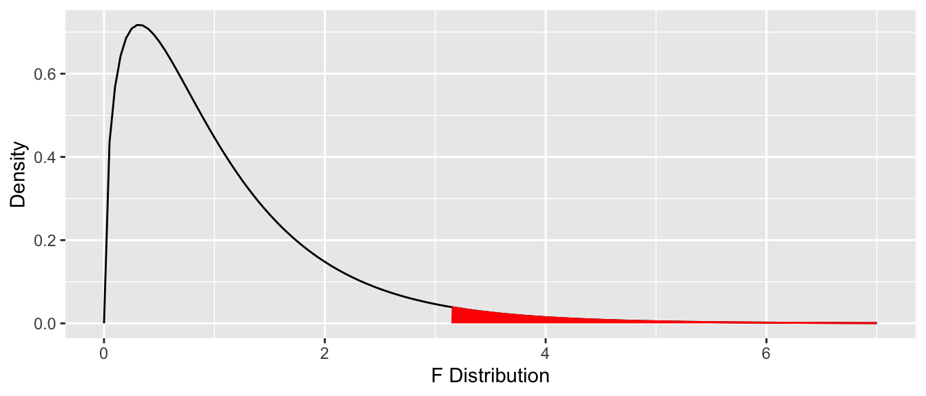
Figure 12.1: ANOVA \(p\)-value is the one-tail area under the \(F\) distribution.
After rejecting the null hypothesis that all of the means are the same, we are often interested in determining which means are different. See Exercise 12.21 for an approach for doing this using Tukey’s Honest Significant Differences method.
12.2.2 Example: Humanization
Different social groups may hold strong opinions about each other. A 2018 study by Davies et al.111 examined American opinions about Pakistanis, and whether those opinions changed when participants learned about humanitarian behavior by Pakistanis. American participants in the study were read a brief synopsis of the tragedy of Hurricane Katrina, and then:
- Told nothing further (the control group).
- Told about the aid sent by Pakistan, and told low numbers for the amount of that aid.
- Told about the aid sent by Pakistan, and told high numbers for the amount of that aid.
Afterwards, the participants were asked how strongly they believed Pakistanis would have felt both primary and secondary emotions following the disaster, and the mean of their responses was taken. The secondary emotions in this study were grief, sorrow, mourning, anguish, guilt, remorse, and resentment.
We plan on analyzing whether there is a difference in the mean of the three groups’ belief of how strongly Pakistanis would have felt secondary emotions. One issue with the technique that we are using is that we are averaging the ordinal scale responses to the seven questions on emotions, which is a common, but not always valid, thing to do.
We can load the data via the following.
humanization <- fosdata::humanizationWe will first examine the data to see whether it appears to be approximately normal with equal variances across the groups. We are only concerned in this problem with the people who were told about Hurricane Katrina.
kat_humanization <- humanization %>%
  filter(stringr::str_detect(group, "Kat"))
ggplot(kat_humanization, aes(x = group, y = pak_sec)) +
  geom_boxplot() +
  geom_jitter(height = 0, width = 0.2)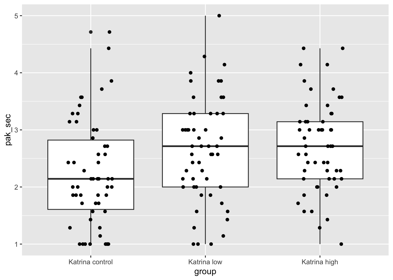
Those don’t look too bad, except that the control group and the low group both have more values exactly equal to 1 than would be expected in a normal distribution. Let’s look at the mean, standard deviation, and sample size in each group.
kat_humanization %>%
  group_by(group) %>%
  summarize(
    mean = mean(pak_sec),
    sd = sd(pak_sec),
    n = n()
  )
## # A tibble: 3 × 4
## group mean sd n
## <fct> <dbl> <dbl> <int>
## 1 Katrina control 2.24 0.927 54
## 2 Katrina low 2.65 0.911 53
## 3 Katrina high 2.72 0.794 54It’s also a good idea to do a histogram.
ggplot(kat_humanization, aes(x = pak_sec)) +
  geom_histogram(bins = 8) +
  facet_wrap(~group)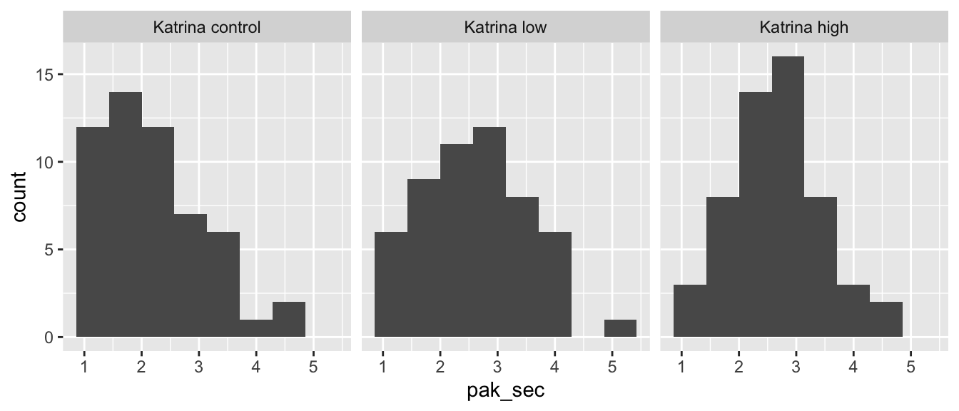
The control group may be moderately right-skewed, but we see nothing that would invalidate a one-way ANOVA analysis.
To perform one-way ANOVA in R, first build a linear model for pak_sec as explained by group, and then apply the anova function to the model.
human_mod <- lm(pak_sec ~ group, data = kat_humanization)
anova(human_mod)
## Analysis of Variance Table
##
## Response: pak_sec
## Df Sum Sq Mean Sq F value Pr(>F)
## group 2 7.456 3.7279 4.8269 0.009231 **
## Residuals 158 122.025 0.7723
## ---
## Signif. codes: 0 '***' 0.001 '**' 0.01 '*' 0.05 '.' 0.1 ' ' 1The ANOVA table gives the \(p\)-value as Pr(>F), here \(p = 0.009231\).
According to the \(p\)-value, we reject \(H_0\) and conclude that not all three of the groups had the same mean.
The test suggests that the story told had an effect on the opinions of the American participants.
12.3 Unequal variance
The equal variances assumption of ANOVA is often difficult to verify. In this section, we introduce a variant of one-way ANOVA that corrects for unequal variance. We then use simulation to explore the effect of unequal variance on the results of one-way ANOVA.
12.3.1 The oneway.test
The function oneway.test operates similarly to one-way ANOVA but performs an approximation procedure
(called Welch’s correction) to correct for unequal variance.
We introduce oneway.test with an example of data involving the greying of chimpanzees.
The fosdata::chimps data comes from a 2020 study by Tapanes et al.112
The investigators showed photographs of chimpanzees to human judges, who rated the greyness of chimpanzee facial hair on a scale of 1-6.
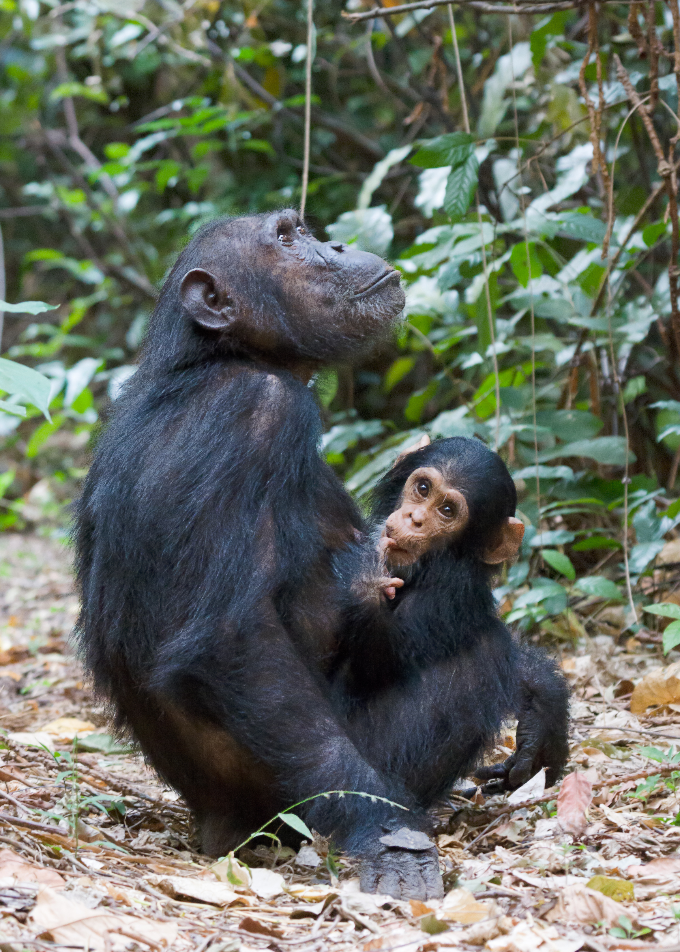
Ikiwaner. GNU Free Documentation License, Version 1.2 https://commons.wikimedia.org/wiki/File:Gombe_Stream_NP_Mutter_und_Kind.jpg
The goal of the study was to determine whether grey hair in chimpanzees increases with age, as it does with humans. The authors found that for chimpanzees aged 30 and older, there does not seem to be an age effect. We will use the data in a different way. The study included chimpanzees from three different locations: the Ngogo community in Uganda, the South community at Taï National Park, Ivory Coast, and the captive population of the New Iberia Research Center (NIRC). We wish to determine whether the mean grey hair is different for chimpanzees in the three groups.
Since the study found no age effect for older chimpanzees, we may ignore age in our analysis if we restrict to chimps aged 30 and older. One chimpanzee, Brownface, has two pictures in the data set. To maintain independence, we arbitrarily chose to remove his 2011 photograph. This choice did not affect the conclusions of our statistical analysis. We load and clean the data first:
old_chimps <- fosdata::chimps %>%
  filter(age >= 30) %>%
  filter(!(individual == "Brownface" & year == 2011))
Next, we make a boxplot to visually compare the three groups.
old_chimps %>%
  ggplot(aes(x = population, y = grey_score_avg)) +
  geom_boxplot()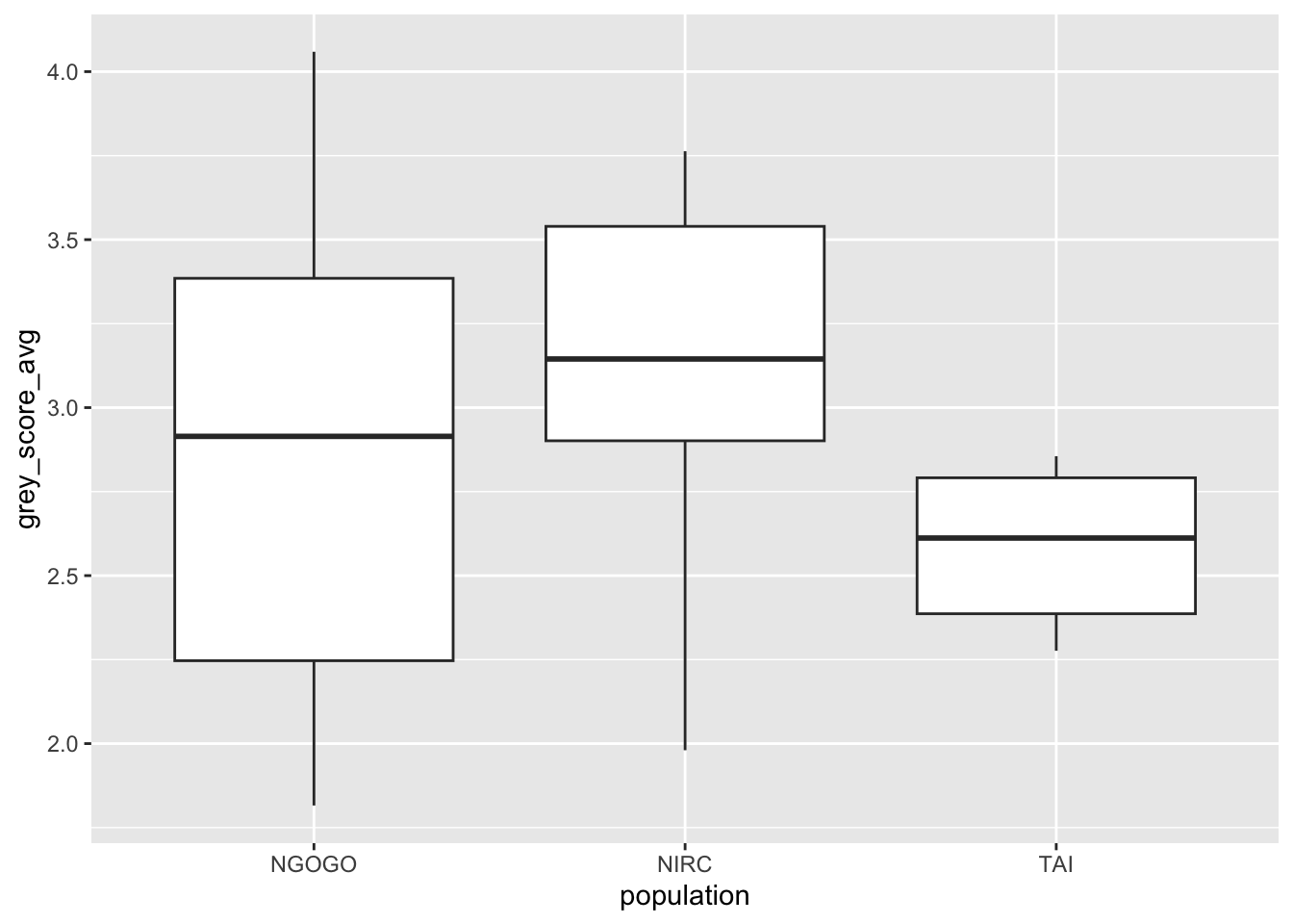
Based on this plot, it appears there may be a difference in mean grey score by population. However, the variances of the three groups are visibly different. The box and whiskers have more spread for NGOGO and less for TAI. Using one-way ANOVA on this data could give misleading results.
The one-way test has the same independence and normality assumptions as one-way ANOVA, and the same null and alternative hypotheses. For the chimps,
\[ H_0: \mu_\text{NGOGO} = \mu_\text{NIRC} = \mu_\text{TAI}, \quad H_a: \text{not all of the $\mu_i$ are equal}. \]
We test grey_score_avg as explained by the factor variable population:
oneway.test(grey_score_avg ~ population, data = old_chimps)##
## One-way analysis of means (not assuming equal variances)
##
## data: grey_score_avg and population
## F = 4.2285, num df = 2.000, denom df = 18.927, p-value = 0.03033The test results in \(p\)-value of \(.03033\), so we reject \(H_0\) at the \(\alpha = 0.05\) level. We conclude that the three groups do not have the same greyness.
Incorrectly using anova in spite of the unequal variance would result in the less reliable value \(p = 0.14\), which
fails to detect a difference among the three groups.
12.3.2 Error simulations
For the chimpanzee data, unequal variance led to a striking difference between the results of one-way ANOVA and the
results of oneway.test. In this section, simulations show how much unequal variances might affect the accuracy of ANOVA.
The simulations in this section assume the underlying populations are normal and independent, but have unequal variances. We will measure the effective type I error rates when \(\alpha = .05\). The results will depend on whether or not our groups have equal or unequal sample sizes – generally the behavior of one-way ANOVA worsens when sample sizes are unequal.
Equal sample sizes
We create three groups of data, each size \(n_i = 30\), all normally distributed with mean 0. Data in the first two groups has standard deviation 1, and in the third group we use standard deviation \(\sigma\). The code below creates a function to run the simulation for various values of \(\sigma\). For each \(\sigma\), it calculates the probability of type I error, where we have \(p < .05\) and incorrectly reject \(H_0\).
sdevs <- c(0.01, 0.05, 0.1, 0.5, 5, 10, 50, 100)

sapply(sdevs, function(sigma) {
  pvals <- replicate(10000, {
    three_groups <- data.frame(
      group = factor(rep(1:3, each = 30)),
      values = rnorm(90, 0, rep(c(1, 1, sigma), each = 30))
    )
    anova(lm(values ~ group, data = three_groups))$`Pr(>F)`[1]
  })
  mean(pvals < 0.05)
})
The simulation takes a considerable time to run for 10,000 trials, and results in the following:
| \(\sigma\) | 0.01 | 0.05 | 0.1 | 0.5 | 5 | 10 | 50 | 100 |
|---|---|---|---|---|---|---|---|---|
| \(P(p < .05)\) | 0.0649 | 0.0639 | 0.0608 | 0.0572 | 0.0779 | 0.0866 | 0.0902 | 0.0911 |
The effective type I error is consistently too high. A correctly functioning test would have type I error of 0.05 in this setting. Things are worse when the third group has large variance, not quite as bad when it has small variance.
Unequal sample sizes
In this simulation, the three groups have sample sizes \(n_1 = 30\), \(n_2 = 30\), and \(n_3\) which will vary from 10 to 500. For each value of \(n_3\), we create data with three groups that are normal, mean 0, and have standard deviation 1, 1, and 5 respectively. In each replication, the \(p\)-value is checked against \(\alpha = 0.05\).
sample_sizes <- c(10, 20, 50, 100, 500)
sapply(sample_sizes, function(n3) {
  pvals <- replicate(10000, {
    three_groups <- data.frame(
      group = factor(rep(1:3, times = c(30, 30, n3))),
      values = rnorm(60 + n3, 0, rep(c(1, 1, 5), times = c(30, 30, n3)))
    )
    anova(lm(values ~ group, data = three_groups))$`Pr(>F)`[1]
  })
  mean(pvals < .05)
})| \(n_3\) | 10 | 20 | 50 | 100 | 500 |
|---|---|---|---|---|---|
| \(P(p < .05)\) | 0.3031 | 0.1483 | 0.0263 | 0.0028 | 0.0000 |
Unequal sample sizes exacerbate the problem! These type I error rates would be 5% if the test were working. When the different group’s sample size is small relative to the other two, the error rate is as high as 30%. This means that 30% of the time, the test detects a difference in means where none exists. This is very bad, because it can lead investigators to find significance when none exists.
When the sample size is large, the rate falls to below 0.01%, indicating the test is failing to work as advertised. This is also bad because it will adversely affect the power of the test in instances where there is a difference in means.
The oneway.test does not depend on equal variances, so it should work properly under the same conditions:
sample_sizes <- c(10, 20, 50, 100, 500)
sapply(sample_sizes, function(n3) {
  pvals <- replicate(10000, {
    three_groups <- data.frame(
      group = factor(rep(1:3, times = c(30, 30, n3))),
      values = rnorm(60 + n3, 0, rep(c(1, 1, 5), times = c(30, 30, n3)))
    )
    oneway.test(values ~ group, data = three_groups)$p.value
  })
  mean(pvals < .05)
})| \(n_3\) | 10 | 20 | 50 | 100 | 500 |
|---|---|---|---|---|---|
| \(P(p < .05)\) | 0.0482 | 0.0490 | 0.0502 | 0.0513 | 0.0489 |
As desired, the effective type I error rate when \(\alpha = .05\) is approximately \(.05\) in all cases.
If you suspect your populations may not follow the assumptions for ANOVA, simulations give a measure of how big a problem it will cause. For example, if you have two samples of size 30 and one of size 10, then you want to be pretty strict about the equal variance assumption. If your sample sizes are all 30, then you don’t need to be as strict.
12.4 Pairwise \(t\)-tests
Suppose we have \(k\) groups of observations and wish to detect a difference in means. It is tempting to perform \(t\)-tests on some or all of the groups, especially if two groups seem quite different. This sort of analysis is problematic because the selection of two groups biases the results. Given enough groups, even if all come from the same population, it is quite likely that two of them will appear to be different.
One approach that avoids the issue of selection is to test all possible pairs. For \(k\) groups, this results in \(\binom{k}{2}\) different \(t\)-tests. The resulting \(p\)-values must be adjusted upward to account for the multiple tests. This method is called pairwise \(t\)-tests.
Pairwise \(t\)-tests have the advantage of showing directly which pairs of groups have significant differences in means. They also apply in experiments where subjects are reused across all groups, when one-way ANOVA is not appropriate due to dependence (see Exercise 12.18).
On the other hand, pairwise \(t\)-tests do not directly test the hypothesis of interest, \(H_0: \mu_1 = \mu_2 = \cdots = \mu_k\) versus \(H_a\): at least one of the means is different. Generally ANOVA will have more power (see Exercise 12.14).
The R command for doing pairwise \(t\)-tests is pairwise.t.test. This function requires two values:
x the measured value or response vector and g the grouping variable.
Perform pairwise \(t\)-tests to determine differences between groups for the mice_pot data set.
pairwise.t.test(mice_pot$percent_of_act, mice_pot$group)##
## Pairwise comparisons using t tests with pooled SD
##
## data: mice_pot$percent_of_act and mice_pot$group
##
## VEH 0.3 1
## 0.3 1.000 - -
## 1 1.000 1.000 -
## 3 0.050 0.124 0.072
##
## P value adjustment method: holmThe only pair approaching significance is the test between the control (VEH) group and the treatment group that received the highest THC dose, 3 mg/kg. With this result, it would be hard to claim a relationship between THC and locomotive impairment. At the start of the chapter, we used ANOVA to calculate a single \(p\)-value of \(0.0357\), somewhat stronger evidence of a difference between the four groups of mice.
Perform pairwise \(t\)-tests to determine differences between groups for the humanization
data set from Section 12.2.2.
pairwise.t.test(kat_humanization$pak_sec, kat_humanization$group)##
## Pairwise comparisons using t tests with pooled SD
##
## data: kat_humanization$pak_sec and kat_humanization$group
##
## Katrina control Katrina low
## Katrina low 0.033 -
## Katrina high 0.013 0.647
##
## P value adjustment method: holmThere is a significant difference at \(\alpha = .05\) between the control and both the low (\(p = 0.033\)) and high (\(p = 0.013\)) levels of aid stories, but no significant difference between the high and low level of aid stories (\(p = 0.647\)). Compare these values with the ANOVA \(p\)-value of 0.009 from Section 12.2.2, which showed an overall difference among the groups.
The pairwise.t.test function has additional options to control its behavior.
p.adjust.method- The method for adjusting the \(p\)-values, which can be “none,” “holm,” and “bonferroni.” These options are explored in the next section.
pool.sd-
Whether we want to pool the standard deviation across all of the groups to get an estimate of the common standard deviation, or whether we estimate the standard deviation of each group separately. Set to
TRUEif we know that the variances of all the groups are equal, or possibly if some of the groups are small. Otherwise,FALSE. paired-
Set to
TRUEif the observations are paired between each group. Default isFALSE. alternative- Used for one-sided tests. The alternate hypothesis for each pair will be that the lower numbered group has a mean strictly less than (or greater than) the higher numbered group. This means that the ordering of groups is important.
12.4.1 FWER and \(p\)-value adjustments
This section investigates the methods for adjusting \(p\)-values when performing multiple tests. First, we define a measure for the failure of multiple tests.
Suppose that multiple hypothesis tests are conducted. The Family Wide Error Rate (FWER) is the probability of making at least one type I error in any of the tests.
Estimate the FWER for an uncorrected pairwise \(t\)-test on six iid groups, each normal with mean 0 and sd 1. Use a sample size of \(n_i = 10\) from each group.
As a first step, generate one set of data and observe the results. In the pairwise \(t\)-test, set p.adjust.method to “none”
so no \(p\)-value correction is performed.
six_groups <- data.frame(
  values = rnorm(60),
  groups = factor(rep(1:6, each = 10))
)
pvals <- pairwise.t.test(six_groups$values,
  six_groups$groups,
  p.adjust.method = "none"
)$p.value
pvals
## 1 2 3 4 5
## 2 0.7694607 NA NA NA NA
## 3 0.5048147 0.3383610 NA NA NA
## 4 0.9769938 0.7475434 0.5233001 NA NA
## 5 0.9961214 0.7731745 0.5017338 0.9731171 NA
## 6 0.9774319 0.7911463 0.4870307 0.9544448 0.9813092By looking at the results, we can tell that none of the 15 \(p\)-values are less than 0.05.
To simulate, we use the any function to detect whether any of the \(p\)-values are less than 0.05, indicating a family-wide error.
sim_data <- replicate(10000, {
  six_groups <- data.frame(
    values = rnorm(60),
    groups = factor(rep(1:6, each = 10))
  )
  pvals <- pairwise.t.test(six_groups$values,
    six_groups$groups,
    p.adjust.method = "none"
  )$p.value
  any(pvals < .05, na.rm = TRUE)
})mean(sim_data)## [1] 0.3582The simulation gives a FWER of 0.3582, so an uncorrected pairwise \(t\)-test would result in a type I error about 36% of the time. A correction to the \(p\)-values for multiple tests is certainly required!
The Bonferroni correction to the pairwise \(t\)-test multiplies each \(p\)-value by the total number of tests, capping \(p\) at 1 if necessary. The Bonferroni correction is a conservative approach, and will lead to a FWER of less than the specified \(\alpha\) level.
Repeating the simulation in Example 12.7 using p.adjust.method = "bonferroni" results in a FWER of about 0.04,
which is indeed less than \(\alpha = .05\).
A more sophisticated technique is the Holm correction.
The FWER of Holm is the same as that of Bonferroni, but in general Holm is more powerful.
For this reason, Holm is the preferred method and the default used by pairwise.t.test.
In Exercise 12.17, you are asked to show that the power of Holm is higher than the power of Bonferroni in a specific instance.
Vignette: Reproducibility
Up to this point in the book, we have emphasized writing reproducible code. Reproducible code means that anyone can take the R script or R Markdown file from a statistical analysis and run it as is to get exactly the results that were reported. This is important because it can often be challenging to understand which exact details were used for a statistical test when reading the summary of an experiment. Providing reproducible code eliminates any confusion about what techniques were used.
A second notion of reproducibility is that of reproducible science. A crucial aspect of the scientific method is that experiments should be reproducible. There is currently a reproducibility crisis in several scientific areas, in the sense that it is believed that many published results would not be reproduced if the experiment was repeated. Here are some reasons for that.
- Significance
- Let’s say that a \(p\)-value less than .05 means that we can reject \(H_0\). Then we will reject \(H_0\) five percent of the time even when it is true. Now, consider how many thousands of statistical tests are run each day. Many (in fact, 5%) of those tests will result in \(p < .05\) simply due to chance. This leads to a problem reproducing significance.
- Power and effect size
- Some experiments do not have a sample size that is large enough to attain a reasonable power. When a test is underpowered and yet \(p < .05\), frequently the effect size gets overestimated. That is, if we are interested not only in whether \(H_0\) is false but also how big of a difference from \(H_0\) there is, we will overestimate that difference in an underpowered test. This leads to a problem reproducing effect sizes. We recommend doing a power analysis whenever possible before collecting data.
- Data dredging
- Some experimenters will take measurements on hundreds or thousands of variables, and look for interesting patterns. If the experimenters do enough tests and check on enough things, then eventually they will find something that is statistically significant. This is fine, as long as the experimenters report all of the tests that they conducted or considered in addition to the ones that were significant. Unethical researchers might not report on the data that wasn’t significant, which is called \(p\)-hacking. Even if researchers report all of the tests that were run, people can be misled by the statistically significant results, and assign them more importance than deserved. Both \(p\)-hacking and misinterpretation lead to reproducibility issues. We recommend reporting all tests that were run (or considered, but not run based on the data). We also recommend making all data and scripts public whenever possible.
- Researcher degrees of freedom
-
There are many decisions that go into collecting and analyzing data. Consider outliers. If we think that data is an outlier or may have been miscoded, it is common practice to check with the person who collected the data. How do we decide what appears to be an outlier? If there are too many, then maybe we use a Wilcoxon rank sum test or other method that is robust to outliers rather than a \(t\)-test. If we are using a \(t\)-test, how do we decide whether
var.equalisTRUEorFALSE? Do you perform a log transformation of the data? Is the alternative hypothesis one-sided or two-sided? There are any number of things that we may or may not do when analyzing a data set, and each one has an effect on the outcome that is hard to quantify. As a solution, we recommend pre-registration. Pre-registration means the experimenters state the details of the data collection and analysis procedure before starting to collect data. Any deviance from the pre-registered procedure should be noted and justified. - Replication incentives
- Replication studies are not seen as exciting and result in little social or financial reward. They are more difficult to publish, since they are not original results. Not surprisingly, replication studies are conducted far less often than original research. The dearth of replication studies has allowed research with statistical design flaws to linger and gain credence, leading to larger crises when the results cannot be reproduced.
Exercises
Exercises 12.1 – 12.3 require material through Section 12.1.
Consider the chimps data set from the fosdata package.
This data set contains 169 observations of (among other things) the average grey hair score grey_score_avg of chimps together with a population that the chimps come from. Suppose that the order of the populations is NIRC, NGOGO, TAI. In the notation of Section 12.1, find \(n_1, n_2, n_3\) as well as \(\overline{x}_{i\cdot}\) for \(i = 1, 2, 3\).
If you have 30 independent observations of 3 groups, each of which is normal with the same mean and standard deviation, what is the distribution of the one-way ANOVA test statistic \(F\)? Include degrees of freedom.
Create a simulation that shows that the one-way ANOVA test statistic follows an \(F\) distribution under the null hypothesis. Assume that you have 4 groups, each with 25 subjects, and each with mean 1 and standard deviation 2. Show via simulation that the ANOVA test statistic \(F\) is an \(F\) random variable with \(k - 1\) and \(N - k\) degrees of freedom.
Exercises 12.4 – 12.8 require material through Section 12.2.
Consider the weight_estimate data in the fosdata package.
Children and adults were asked to estimate the weight of an object that an actor picks up. Conduct a one-way ANOVA test at the \(\alpha = .05\) level to test whether the means of the weight estimates for the 300 g object are the same across the age groups in the study.
Consider the case0502 data from Sleuth3. Dr. Benjamin Spock was tried
in Boston for encouraging young men not to register for the draft.
It was conjectured that the judge in Spock’s trial did not have appropriate representation of women.
The jurors were supposed to be selected by taking a random sample of 30 people (called venires), from which the jurors would be chosen. In the data case0502, the percent of women in 7 judges’ venires are given.
- Create a boxplot of the percent women for each of the 7 judges. Comment on whether you believe that Spock’s lawyers might have a point.
- Determine whether there is a significant difference in the percent of women included in the 6 judges’ venires who aren’t Spock’s judge.
- Determine whether there is a significant difference in the percent of women induced in Spock’s venires versus the percent included in the other judges’ venires combined. (Your answer to part (b) should justify doing this.)
Consider the data in ex0524 in Sleuth3.
This gives 2584 data points, where each subject’s IQ was measured in 1979 and their income was measured in 2005. Create a boxplot of income for each of the IQ quartiles. Is there evidence to suggest that there is a difference in mean income among the 4 groups of IQ? Check the assumptions necessary to do one-way ANOVA. Does this cause you to doubt your result?
The built-in data set chickwts measures weights of chicks after six weeks eating various types of feed.
Test if the mean weight is the same for all feed types. Are the assumptions for one-way ANOVA reasonable?
The data set MASS::immer from the MASS package has data on a trial of barley varieties performed by
Immer, Hayes, and Powers in the early 1930’s. Test if the total yield (sum of 1931 and 1932) depends on the variety of barley.
Are the assumptions for ANOVA reasonable?
Exercises 12.9 – 12.13 require material through Section 12.3.
The built-in data set InsectSprays records the counts of living insects in agricultural experimental units treated with different insecticides.
- Plot the data. Three of the sprays seem to be more effective (less insects collected) than the other three sprays. Which three are the more effective sprays?
- Use one-way ANOVA to test if the three effective sprays have the same mean. What do you conclude?
- Use one-way ANOVA to test if the three less effective sprays have the same mean. What do you conclude?
- Would it be appropriate to use one-way ANOVA on the entire data set? Why or why not?
- Use
oneway.testto test the null hypothesis that all of the mean insect counts are the same for the various sprays versus the alternative that they are not, at the \(\alpha = .01\) level.
The built-in data set morley gives speed of light measurements for five experiments done by Michelson in 1879.
- Create a boxplot with one box for each of the five experiments.
- Compute the sample standard deviation and sample size for each of the five experiments.
- Use ANOVA to test if the five experiments have the same mean, and report your findings. Careful: the
Exptvariable is coded as an integer. - Use
oneway.testto test if the five experiments have the same mean, and report your findings.
The msleep data set in the ggplot2 package has information about 83 species of mammals.
- How many mammal species are in each
voregroup? - Make a boxplot to show how
sleep_totaldepends onvore. - The group variances are apparently unequal, so use
oneway.testto test if the mean sleep total depends on vore. - Run the ANOVA anyway. What \(p\) value does it report?
Notice that the unequal variance combined with unequal group sizes made a huge difference in the \(p\)-value.
Estimate the effective type I error rate when performing one-way ANOVA on 4 groups at the \(\alpha = .05\) level. Assume groups 1-3 are size 20 and group 4 is size 100. Assume all groups have mean 0, groups 1-3 have standard deviation 1, and group 4 has standard deviation 2.
Repeat Exercise 12.12, but assume all groups have size 20. Is the effective type I error closer to the \(\alpha = .05\) level, or further from it?
Exercises 12.14 – 12.22 require material through Section 12.4.
Suppose you have 6 groups of 15 observations each. Groups 1-3 are normal with mean 0 and standard deviation 3, while groups 4-6 are normal with mean 1 and standard deviation 3. Compare via simulation the power of the following tests of \(H_0: \mu_1 = \dotsb = \mu_6\) versus the alternative that at least one pair is different at the \(\alpha = .05\) level.
- One-way ANOVA. (Hint:
anova(lm(formula, data))[1,5]pulls out the \(p\)-value of ANOVA.) pairwise.t.test, where we reject the null hypothesis if any of the paired \(p\)-values are less than 0.05.
The next two exercises use the data set flint from the fosdata package.
The data set fosdata::flint contains data on lead levels in water samples taken from Flint, Michigan, during the “Flint water crisis” of 2015.
Three lead measurements were taken at each house, Pb1, Pb2, and Pb3, on first draw, after 45 seconds, and after 2 minutes of water running.
As observed in 9.16, the lead levels are highly skew.
- Make a boxplot showing the distribution of the log levels of Pb1 for each ward. Notice that ward 0 contains only a single sample. In fact, there is no ward 0 in Flint. Remove that data point before continuing.
- Do the log Pb1 levels for each ward appear normally distributed? Are the variances approximately equal across wards?
- Use ANOVA to determine if there is a difference in log Pb1 levels across the wards of Flint. Report a \(p\)-value with your answer.
- Make a boxplot showing the distribution of the log levels of Pb1, Pb2, and Pb3. Hint: use
pivot_longerto tidy the data. - Do the three log levels appear normally distributed? Are their variances approximately equal?
- Explain why it is inappropriate to use one-way ANOVA to test for a difference among the means of the three log lead levels.
- Use a pairwise \(t\)-test to determine if there is a difference in log lead level between the first draw, 45 second, and 2 minute samples.
Suppose you have three populations, all of which are normal with standard deviation 1, and with means \(0\), \(0.5\), and \(1\). You take samples of size 30 and perform a pairwise \(t\)-test.
- Estimate the percentage of times that at least one of the null hypotheses being tested is rejected when using the “bonferroni” \(p\)-value adjustment.
- Estimate the percentage of times that at least one of the null hypotheses being tested is rejected when using the “holm” \(p\)-value adjustment.
Consider the data set cows_small in the fosdata package. In this data set, cows in Davis, CA were sprayed with water on hot days to try to cool them down. Each cow was measured with no spray (control), nozzle TK-0.75, and nozzle TK-12.
- Is one-way ANOVA appropriate to use on this data set? If so, do it. If not, explain why not.
- Perform pairwise \(t\)-tests on the three groups with
holm\(p\)-value adjustment and explain.
Suppose you perform pairwise \(t\)-tests on \(6\) iid groups.
- How many tests are required?
- At the \(\alpha = 0.05\) level, what is the probability of type I error for a single one of these tests?
- Assume the pairwise tests are independent. Compute the exact probability that a type I error occurs on at least one of these tests.
- Compare your answer from part (c) to results of the simulation in Example 12.7. Are the pairwise tests independent?
Consider the weight_estimate data in the fosdata package. Children and adults were asked to estimate the weight of an object that an actor picks up. In Exercise 12.4, you conducted an ANOVA test at the \(\alpha = .05\) level to test whether the means of the weight estimates for the 300 g object are the same across the age groups in the study. Use pairwise.t.test to test all pairs of means at the \(\alpha = .05\) level.
Consider the frogs data set in the fosdata package. This data set contains measurements from 6 species of frogs, including one new species, dakha, that the authors of the paper found. When establishing that a group of animals is a new species, it can be important to find physiological differences between the group of animals and animals that are nearest genetically. Read more about the data set by typing ?fosdata::frogs.
- Create a boxplot of the distance from front of eyes to the nostril versus species. Does it appear that the data satisfies the assumptions for one-way ANOVA?
- Test \(H_0\) (all of the mean distances of the species are the same) versus \(H_a\) (not all of the mean distances of the species are the same) at the \(\alpha = .05\) level.
- If you reject \(H_0\), look up
TukeyHSDin base R, and use it to perform a post-hoc analysis to determine which pairs of mean bill depths are the same, and which are different at the \(\alpha = .05\) level. The functionTukeyHSDrequires ANOVA to be done with the following command:mod_aov <- aov(en ~ species, data = frogs). Write up your result in an organized fashion with explanations.
Consider the penguins data set in the palmerpenguins package that was discussed in Chapter 11.
- Create a boxplot of the variable
bill_depth_mmbyspecies. Does it appear that the data satisfies the assumptions for one-way ANOVA? - Test \(H_0\) (all of the mean bill depths of the species are the same) versus \(H_a\) (not all of the mean bill depths are the same) at the \(\alpha = .01\) level.
- If you reject \(H_0\), perform a post-hoc analysis as in Exercise 12.21 to determine which pairs of mean bill depths are the same, and which are different at the \(\alpha = .01\) level.
Xavier Viñals et al., “Cognitive Impairment Induced by Delta9-Tetrahydrocannabinol Occurs Through Heteromers Between Cannabinoid CB1 and Serotonin 5-HT2A Receptors,” PLOS Biology 13, no. 7 (July 2015): e1002194.↩︎
This quantity is often denoted \(SS_W\), but we choose \(SS_R\) to match the R output, where it is denoted as the sum of squares of residuals.↩︎
Thomas Davies et al., “From Humanitarian Aid to Humanization: When Outgroup, but Not Ingroup, Helping Increases Humanization,” PLOS One 13, no. 11 (2018): e0207343.↩︎
Elizabeth Tapanes et al., “Does Facial Hair Greying in Chimpanzees Provide a Salient Progressive Cue of Aging?” PLOS One 15, no. 7 (2020): e0235610.↩︎