Chapter 2 Probability
A primary goal of statistics is to describe the real world based on limited observations. These observations may be influenced by random factors, such as measurement error or environmental conditions. This chapter introduces probability, which is designed to describe random events. Later, we will see that the theory of probability is so powerful that we intentionally introduce randomness into experiments and studies so we can make precise statements from data.
2.1 Probability basics
In order to learn about probability, we must first develop a vocabulary that we can use to discuss various aspects of it.
Terminology for statistical experiments:
- An experiment is a process that produces an observation.
- An outcome is a possible observation.
- The set of all possible outcomes is called the sample space.
- An event is a subset of the sample space.
- A trial is a single running of an experiment.
Roll a die and observe the number of dots on the top face. This is an experiment, with six possible outcomes. The sample space is the set \(S = \{1,2,3,4,5,6\}\). The event “roll higher than 3” is the set \(\{4,5,6\}\).
Stop a random person on the street and ask them in which month they were born. This experiment has the twelve months of the year as possible outcomes. An example of an event \(E\) might be that they were born in a summer month, \(E = \{\text{June}, \text{July}, \text{August}\}\).
Suppose a traffic light stays red for 90 seconds each cycle. While driving you arrive at this light, and observe the amount of time that you are stopped until the light turns green. The sample space is the interval of real numbers \([0,90]\). The event “you didn’t have to stop” is the set \(\{0\}\).
Since events are, by their very definition, sets, it will be useful for us to review some basic set theory.
Let \(A\) and \(B\) be events in a sample space \(S\).
- \(A \cap B\) is the set of outcomes that are in both \(A\) and \(B\).
- \(A \cup B\) is the set of outcomes that are in either \(A\) or \(B\) (or both).
- \(A - B\) is the set of outcomes that are in \(A\) and not in \(B\).
- The complement of \(A\) is \(\overline{A} = S - A\). So, \(\overline{A}\) is the set of outcomes that are not in \(A\).
- The symbol \(\emptyset\) is the empty set, the set with no outcomes.
- \(A\) and \(B\) are disjoint if \(A \cap B = \emptyset\).
- \(A\) is a subset of \(B\), written \(A \subset B\), if every element of \(A\) is also an element of \(B\).
Suppose that the sample space \(S\) consists of the positive integers. Let \(A\) be the set of all positive even numbers, and let \(B\) be the set of all prime numbers. Then, \(A = \{2, 4, 6, \ldots\}\) and \(B = \{2, 3, 5, 7, 11, \ldots\}\). Then,
- \(A \cap B = \{2\}\)
- \(A \cup B = \{2, 3, 4, 5, 6, 7, 8, 10, 11, 12, 13, 14, 16, 17, 18, 19, 20, 22, \ldots\}\)
- \(B - A\) is the set of odd prime numbers.
- \(\overline{A}\) is the set of all positive odd integers.
- \(A\) and \(B\) are not disjoint, since both contain the number 2.
- \(A\) is not a subset of \(B\) since \(4\) is in \(A\), but 4 is not an element of \(B\).
The probability of an event is a number between zero and one that describes the proportion of time we expect the event to occur. Since probability lies at the heart of all mathematical statements in this book, we will define it formally in Definition 2.7 and prove its basic properties in Theorem 2.1.
Let \(S\) be a sample space. A valid probability satisfies the following probability axioms:
- Probabilities are non-negative real numbers. That is, for all events \(E\), \(P(E) \ge 0\).
- The probability of the sample space is 1, \(P(S) = 1\).
- Probabilities are countably additive: If \(A_1, A_2, \ldots\) are pairwise disjoint, then \[ P\left(\bigcup_{n=1}^\infty A_n\right) = \sum_{n= 1}^\infty P(A_n) \]
We will not be concerned in this book about carefully describing all of the subsets of \(S\) which have an associated probability. We will assume that any event of interest will be an event associated with a probability.
Probabilities obey some important rules, which are consequences of the axioms.
Let \(A\) and \(B\) be events in the sample space \(S\).
- \(P(\emptyset) = 0\).
- If \(A\) and \(B\) are disjoint, then \(P(A \cup B) = P(A) + P(B)\).
- If \(A \subset B\), then \(P(A) \le P(B)\).
- \(0 \le P(A) \le 1\).
- \(P(A) = 1 - P(\overline{A})\).
- \(P(A - B) = P(A) - P(A \cap B)\).
- \(P(A \cup B) = P(A) + P(B) - P(A \cap B)\).
We sketch the proof of these results. Part 1 follows from countable additivity. Let \(A_1, A_2, \ldots\) all be the empty set. Since they are pairwise disjoint, \(P(\emptyset) = \sum_{i = 1}^\infty P(\emptyset)\), which implies \(P(\emptyset) = 0\). Part 2 is just a special case of probability Axiom 3 with \(A_1 = A\), \(A_2 = B\), and \(A_3,A_4,\dotsc\) all equal to the empty set.
Part 3 follows from letting \(A_1 = A\) and \(A_2 = B - A\) and applying part 2 and Axiom 1. Part 4 follows from parts 1 and 3, together with Axiom 2.
For part 6, we have that \(A = (A \cap B) \cup (A - B)\), where \(A \cap B\) and \(A - B\) are disjoint. We have \(P(A) = P(A \cap B) + P(A - B)\), which gives the result. Part 5 is a special case of part 6.
To prove part 7, we note that \(A \cup B = A \cup (B - A)\), where \(A\) and \(B - A\) are disjoint. Therefore, \(P(A \cup B) = P(A) + P(B - A) = P(A) + P(B) - P(A \cap B)\) by parts 2 and 5.
One way to assign probabilities to events is empirically, by repeating an experiment many times and observing the proportion of times the event occurs. While this can only approximate the true probability, it is sometimes the only approach possible. For example, in the United States, the probability of being born in September is noticeably higher than the probability of being born in January, and these values can only be estimated by observing actual patterns of human births.
Another method is to make an assumption that all outcomes are equally likely, usually because of some physical property of the experiment. When all outcomes are equally likely, we compute the probability of an event \(E\) by counting the number of outcomes in \(E\) and dividing by the number of outcomes in the sample space. Given an event \(E\), we denote the number of outcomes in \(E\) by \(|E|\).
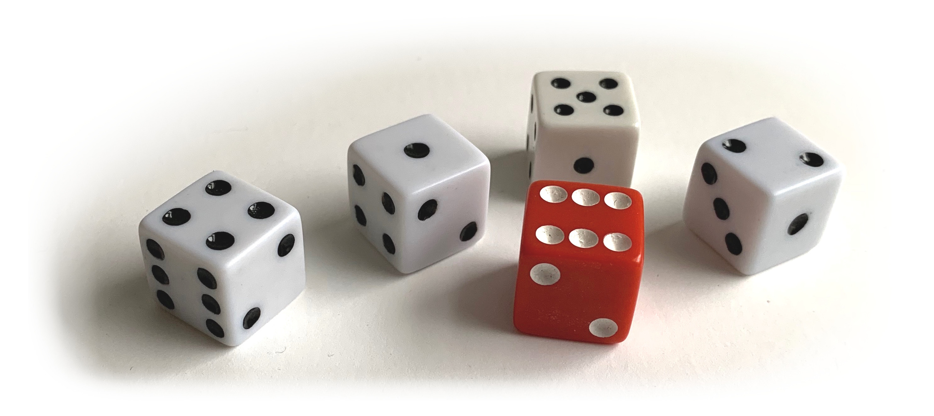
For example, because (high quality) dice are close to perfect cubes, one believes that all six sides of a die are equally likely to occur.
Using the additivity of disjoint events (axiom 3 in the definition of probability),
\[ P(\{1\}) + P(\{2\}) + P(\{3\}) + P(\{4\}) + P(\{5\}) + P(\{6\}) = P(\{1,2,3,4,5,6\}) = 1 \]
Since all six probabilities are equal and sum to 1, the probability of each face occurring is \(1/6\). In this case, the probability of an event \(E\) can be computed by counting the number of elements in \(E\) and dividing by the number of elements in \(S\).
Suppose that two six-sided dice are rolled and the numbers appearing on the dice are observed.8
The sample space \(S\) is given by
\[ \begin{pmatrix} (1,1), (1,2), (1,3), (1,4), (1,5), (1,6) \\ (2,1), (2,2), (2,3), (2,4), (2,5), (2,6) \\ (3,1), (3,2), (3,3), (3,4), (3,5), (3,6) \\ (4,1), (4,2), (4,3), (4,4), (4,5), (4,6) \\ (5,1), (5,2), (5,3), (5,4), (5,5), (5,6) \\ (6,1), (6,2), (6,3), (6,4), (6,5), (6,6) \end{pmatrix} \]
- By the symmetry of the dice, we expect all 36 possible outcomes to be equally likely. So the probability of each outcome is \(1/36\).
- The event “The sum of the dice is 6” is represented by \[ E = \{(1,5), (2,4), (3,3), (4,2), (5,1)\} \]
- The probability that the sum of two dice is 6 is given by \[ P(E) = \frac{|E|}{|S|} = \frac{5}{36}, \] which can be obtained by simply counting the number of elements in each set above.
- Let \(F\) be the event “At least one of the dice is a 2.” This event is represented by \[ F = \{(2,1), (2,2), (2,3), (2,4), (2,5), (2,6), (1,2), (3,2), (4,2), (5,2), (6,2)\} \] and the probability of \(F\) is \(P(F) = \frac{11}{36}\).
- \(E \cap F = \{(2,4), (4,2)\}\) and \(P(E \cap F) = \frac{2}{36}\).
- \(P(E \cup F) = P(E) + P(F) - P(E \cap F) = \frac{5}{36} + \frac{11}{36} - \frac{2}{36} = \frac{14}{36}\).
- \(P(\overline{E}) = 1 - P(E) = \frac{31}{36}\).
What is a probability, actually? Broadly speaking there are two interpretations of probability, known as frequentist and evidential.
The frequentist interpretation: if the probability of an event \(E\) is \(p\), then if you repeat the experiment many times, then the proportion of times that the event occurs will eventually be close to \(p\).
The evidential interpretation: the probability of an event measures the degree of certainty that a person has about whether the event occurs or not.
Both interpretations are reasonable. To understand the difference, consider the following thought experiment. Suppose that I am about to toss a coin, and I ask you to estimate the probability that the coin will land on heads. Not knowing any reason to think otherwise, you might say that you estimate it to be \(p = 0.5\). From the frequentist point of view, that would mean that you believe that if I repeat the experiment infinitely many times, then the proportion of times that it is heads will converge to 0.5. From the certainty of belief point of view, you believe that each outcome (heads/tails) is equally likely.
Now, suppose that I flip the coin and look at it, but don’t tell you whether it is heads or tails. At this point there is nothing random that I can repeat, so the frequentist interpretation cannot assign a probability to the result. However, your degree of certainty about the outcome hasn’t changed, it is still \(p = 0.5\). This example illustrates the importance of the random nature of statistical experiments.
Sometimes, probabilities are discussed in terms of odds. The odds of an event \(E\) are \(\frac{P(E)}{1-P(E)}\), the ratio of the probability of the event occurring to the probability of the event not occurring. Often these are expressed as a ratio with a colon. For example, the probability of rolling a six on a six-sided die is \(1/6\), the probability of not rolling a six is \(5/6\), and the odds of rolling a six are given as \(1\!:\!5\), or “one to five.”
2.2 Simulations
The goal of probability and statistics is to understand the real world. Statistical experiments in the real world are usually slow and often expensive. Instead of running real world experiments, it is easier to model these experiments and then use a computer to imitate the results. This process goes by several names, such as stochastic simulation, Monte Carlo simulation or probability simulation. Since this is the only type of simulation we discuss in this book, we simply call it simulation.
The foundational mathematical theorem which justifies using simulations to estimate probabilities as described in this chapter and throughout the book is the Law of Large Numbers, which is described in detail in this context in Section 2.2.2, and in more generality in Section 3.2.
This book places simulation at the center of the study of probability. With a good understanding of how to simulate experiments, you can answer a wide range of questions involving probability. Later in the book, we will use simulation to explore how statistical methods behave under different assumptions about data. Simulation also plays a fundamental role in modern statistical methods such as resampling, bootstrapping, non-parametric statistics, and genetic algorithms.
2.2.1 Simulation with sample
For an experiment with a finite sample space \(S = \{x_1, x_2, \dotsc, x_n\}\), the R command sample()
can simulate one or many trials of the experiment. Essentially, sample treats \(S\) as a bag of outcomes, reaches into the bag, and picks one.
The syntax of sample is
sample(x, size, replace = FALSE, prob = NULL)
where the parameters are:
x- The vector of elements from which you are sampling.
size- The number of samples you wish to take.
replace-
Whether you are sampling with replacement or not. Sampling without replacement means that
samplewill not pick the same value twice, and this is the default behavior. Passreplace = TRUEto sample if you wish to sample with replacement. prob-
A vector of probabilities or weights associated with
x. It should be a vector of nonnegative numbers of the same length asx. If the sum ofprobis not 1, it will be normalized. If this value is not provided, then each element ofxis considered to be equally likely.
The most straightforward use of sample is to choose one element of a vector “at random.” When people say “at random,” they usually mean that all
outcomes are equally likely to be chosen, and that is how sample operates. To get a random number from 1 to 10:
sample(x = 1:10, size = 1)## [1] 2The size argument tells sample how many random numbers you want:
sample(x = 1:10, size = 8)## [1] 9 10 1 5 6 3 7 2Observe that the eight numbers chosen are all different.
Unless you tell it otherwise, sample will never choose the same outcome twice.
If you ask sample for more than ten different numbers from 1 to 10, you get an error:
sample(x = 1:10, size = 30)## Error in sample.int(length(x), size, replace, prob): cannot take a
## sample larger than the population when 'replace = FALSE'The replace argument of sample determines whether sample is allowed to repeat values. The name “replace” comes from the model that sample has a bag of outcomes and is reaching into the bag to draw one. When replace = FALSE, the default, once sample chooses a value from the bag of outcomes it won’t replace it into the bag. With replace = TRUE, sample draws an outcome from the bag, records it, and then puts it back into the bag.
Here we set replace = TRUE to get 20 random numbers from 1 to 10:
sample(x = 1:10, size = 20, replace = TRUE)## [1] 10 5 10 5 9 6 10 5 10 10 3 1 10 6 8 7 6 2 9 10For sample and many other functions in R, you are not required to name the arguments with x = ... or size = ... as long as these come first and second in the function. For example:
sample(1:10, 20, replace = TRUE)## [1] 10 4 8 8 4 4 8 6 5 3 8 3 2 4 8 1 2 10 1 6However, it is often clearer to explicitly name the arguments to complicated functions like sample. Use your best judgment, and include the parameter name if there is any doubt.
The prob argument of sample allows for sampling when outcomes are not all equally likely.
In the United States, human blood comes in four types: O, A, B, and AB. These types occur with the following probability distribution: \[ \begin{array}{lcccc} \text{Type} &A& AB & B & O\\ \text{Probability} & 0.40 & 0.04 & 0.11 & 0.45 \end{array} \] We can sample thirty blood types from this distribution by defining a vector of blood types and a vector of their probabilities:
bloodtypes <- c("O", "A", "B", "AB")
bloodprobs <- c(0.45, 0.40, 0.11, 0.04)
sample(x = bloodtypes, size = 30, prob = bloodprobs, replace = TRUE)
## [1] "A" "O" "AB" "A" "O" "A" "A" "O" "O" "O" "O" "A" "O"
## [14] "A" "A" "A" "B" "A" "A" "B" "A" "O" "O" "A" "A" "O"
## [27] "O" "A" "A" "O"Observe that a large sample reproduces the original probabilities with reasonable accuracy:
sim_data <- sample(
  x = bloodtypes, size = 10000,
  prob = bloodprobs, replace = TRUE
)
table(sim_data)
## sim_data
## A AB B O
## 3998 425 1076 4501table(sim_data) / 10000## sim_data
## A AB B O
## 0.3998 0.0425 0.1076 0.45012.2.2 Using simulation to estimate probabilities
The goal of simulation is usually to estimate the probability of an event. This is a three-step process:
- Simulate the experiment many times to produce a vector of outcomes.
- Test if the outcomes are in the event to produce a vector of TRUE/FALSE.
- Compute the
meanof the TRUE/FALSE vector to compute the probability estimate.
Steps 1 and 2 can often be interesting problems, and their solutions can require creativity and expertise. Step 3 relies on the fact that
R converts TRUE to 1 and FALSE to 0 when taking the mean of a vector. If we take the average of a vector of TRUE/FALSE values,
we get the number of TRUE divided by the size of the vector, which is exactly the proportion
of times that the event occurred. The theoretical justification for this procedure is given in Theorem 2.2 below.
We illustrate this process by reworking Example 2.8 using simulation.
Suppose that two six-sided dice are rolled and the numbers appearing on the dice are added.
Simulate this experiment by performing 10,000 rolls of each die with sample and then adding the two dice:
die1 <- sample(x = 1:6, size = 10000, replace = TRUE)
die2 <- sample(x = 1:6, size = 10000, replace = TRUE)
sumDice <- die1 + die2
Let’s take a look at the simulated data:
head(die1)## [1] 1 4 1 2 5 3head(die2)## [1] 1 6 1 4 1 3head(sumDice)## [1] 2 10 2 6 6 6Let \(E\) be the event “the sum of the dice is 6,” and \(F\) be the event “at least one of the dice is a 2.” We define these events from our simulated data:
eventE <- sumDice == 6
head(eventE)
## [1] FALSE FALSE FALSE TRUE TRUE TRUEeventF <- die1 == 2 | die2 == 2
head(eventF)## [1] FALSE FALSE FALSE TRUE FALSE FALSEHere, \(F\) is interpreted as “die 1 is a two or die 2 is a two” and uses R’s “or” operator |.
From theory, \(P(E) = \frac{5}{36} \approx 0.139\), and \(P(F) = \frac{11}{36} \approx 0.306\).
Using mean we find out what percentage of the time our events occurred in the simulation,
which estimates the correct probabilities:
mean(eventE) # P(E)## [1] 0.1409mean(eventF) # P(F)## [1] 0.2998To estimate \(P(E \cap F) = \frac{2}{36} \approx 0.056\) we use R’s “and” operator &:
mean(eventE & eventF)## [1] 0.0587It is not necessary to store the TRUE/FALSE vectors in event variables. Here is an estimate of \(P(E \cup F) = \frac{14}{36} \approx 0.389\):
mean((sumDice == 6) | (die1 == 2 | die2 == 2))## [1] 0.382The justification for using simulation to estimate probabilities is given by the following theorem, which in this context is sometimes referred to as Bernoulli’s Theorem. It is a consequence of the more general Law of Large Numbers, Theorem 3.2.
Let \(E\) be an event with probability \(p\). Let \(m_n\) be the number of times that \(E\) occurs in \(n\) repeated trials, where we assume the outcome of trials do not affect the outcome of other trials. Then \[ \lim_{n \to \infty} \frac{m_n}{n} = p. \]
While we cannot simulate running infinitely many trials, we can take a large number of trials and expect that the proportion of successes will be approximately the true probability \(p\). We also expect that a larger number of trials will, on average, give a better estimate of the true probability than a smaller number of trials. We investigate this further in Example 2.13.
2.2.3 Using replicate to repeat experiments
The size argument to sample allowed us to perform many repetitions of an experiment.
For more complicated statistical experiments, we use the R function replicate, which
can take a single R expression and repeat it many times.
The function replicate is an example of an implicit loop in R.
Suppose that expr is one or more R commands, the last of which returns a single value. The call
replicate(n, expr)
repeats the expression stored in expr n times and stores the resulting values as a vector.
Estimate the probability that the sum of seven dice is larger than 30.
To simulate this event once, we can use sample to roll seven dice, sum to add them, and then test for the event “the sum is larger than 30”:
dice <- sample(x = 1:6, size = 7, replace = TRUE) # roll seven dice
sum(dice) > 30 # test if the event occurred
## [1] FALSEThe result of this single simulation was FALSE. Using replicate repeats the experiment many times:
replicate(20, {
  dice <- sample(x = 1:6, size = 7, replace = TRUE) # roll seven dice
  sum(dice) > 30 # test if the event occurred
})
## [1] FALSE FALSE FALSE FALSE FALSE FALSE FALSE TRUE FALSE TRUE FALSE
## [12] FALSE FALSE FALSE FALSE FALSE TRUE FALSE FALSE FALSEThe curly braces { and } are required to replicate more than one R command. When you put multiple commands inside {} you are creating a
code block. A code block acts like a single statement, and only the result of the last command is saved in the vector via replicate.
Using multiple lines for a code block is not required but highly recommended for readability. It is also legal to put the entire code block on a single line and separate each command in the block with a semicolon.
Finally, we want to compute the probability of the event. We replicate 10,000 times for a reasonably accurate estimate:
event <- replicate(10000, {
  dice <- sample(x = 1:6, size = 7, replace = TRUE) # roll seven dice
  sum(dice) > 30 # test if the event occurred
})
mean(event)
## [1] 0.0963When rolling seven dice, there is about a 9.63% probability the sum will be larger than 30. How accurate is our estimate? It is often a good idea to repeat a simulation a couple of times to get an idea about how much variance there is in the results. Running the code a few more times gave answers 0.0947, 0.091, 0.0965, and 0.0867. It seems safe to report the answer as roughly 9%.
The more replications you perform with replicate(), the more accurate you can expect your simulation to be. On the other hand, replications can be slow.
For events which are not rare, 10,000 trials runs quickly and gives an answer accurate to about two decimal places.
For complicated simulations, we strongly recommend that you follow the workflow as presented above; namely,
Write code that performs the experiment a single time.
Replicate the experiment a small number of times and check the results:
replicate(100, { EXPERIMENT GOES HERE }))Replicate the experiment a large number of times and store the result:
event <- replicate(10000, { EXPERIMENT GOES HERE }))Compute probability using
mean(event).
It is much easier to trouble-shoot your code this way, as you can test each line of your simulation separately.
Three dice are thrown. Estimate the probability that the largest value is a four.
Here is one trial:
die_roll <- sample(1:6, 3, TRUE)
max(die_roll) == 4
## [1] TRUEHere are a few trials, and we observe that sometimes the event occurs and sometimes it does not:
replicate(20, {
  die_roll <- sample(1:6, 3, TRUE)
  max(die_roll) == 4
})
## [1] FALSE FALSE FALSE FALSE FALSE FALSE FALSE FALSE FALSE FALSE FALSE
## [12] FALSE FALSE FALSE FALSE TRUE TRUE FALSE FALSE FALSEFinally, perform many trials and compute the probability of the event:
event <- replicate(10000, {
  die_roll <- sample(1:6, 3, TRUE)
  max(die_roll) == 4
})
mean(event)
## [1] 0.1737When three dice are thrown, the probability that the largest value is four is approximately 17%.
The purpose of this example is to investigate the rate at which the proportion of successes converges to the true probability in a specific setting. To do so, we need to choose an experiment and an event \(E\) for which we know \(P(E)\).
Suppose two dice are rolled. Let \(E\) denote the event that the sum of the dice is six. By counting, we know that \(P(E) = 5/36 \approx .138888\). If we use 10 trials to estimate the probability, then the closest we can get is 0.1. We recommend running the code below several times to see that we sometimes get 0.1, but many times also get 0, 0.2 or 0.3.
mean(replicate(10, {
  sum(sample(1:6, 2, T)) == 6
}))
## [1] 0.3On the other hand, when we use 200 trials, we are unlikely to be wrong in the first significant digit.
mean(replicate(200, {
  sum(sample(1:6, 2, T)) == 6
}))
## [1] 0.135If we increase to 10,000 trials, we are even closer on average.
mean(replicate(10000, {
  sum(sample(1:6, 2, T)) == 6
}))
## [1] 0.1413In Figure 2.1, we estimated the probability of \(E\) for simulations ranging from 10 trials to 10,000 trials and then plotted the results.
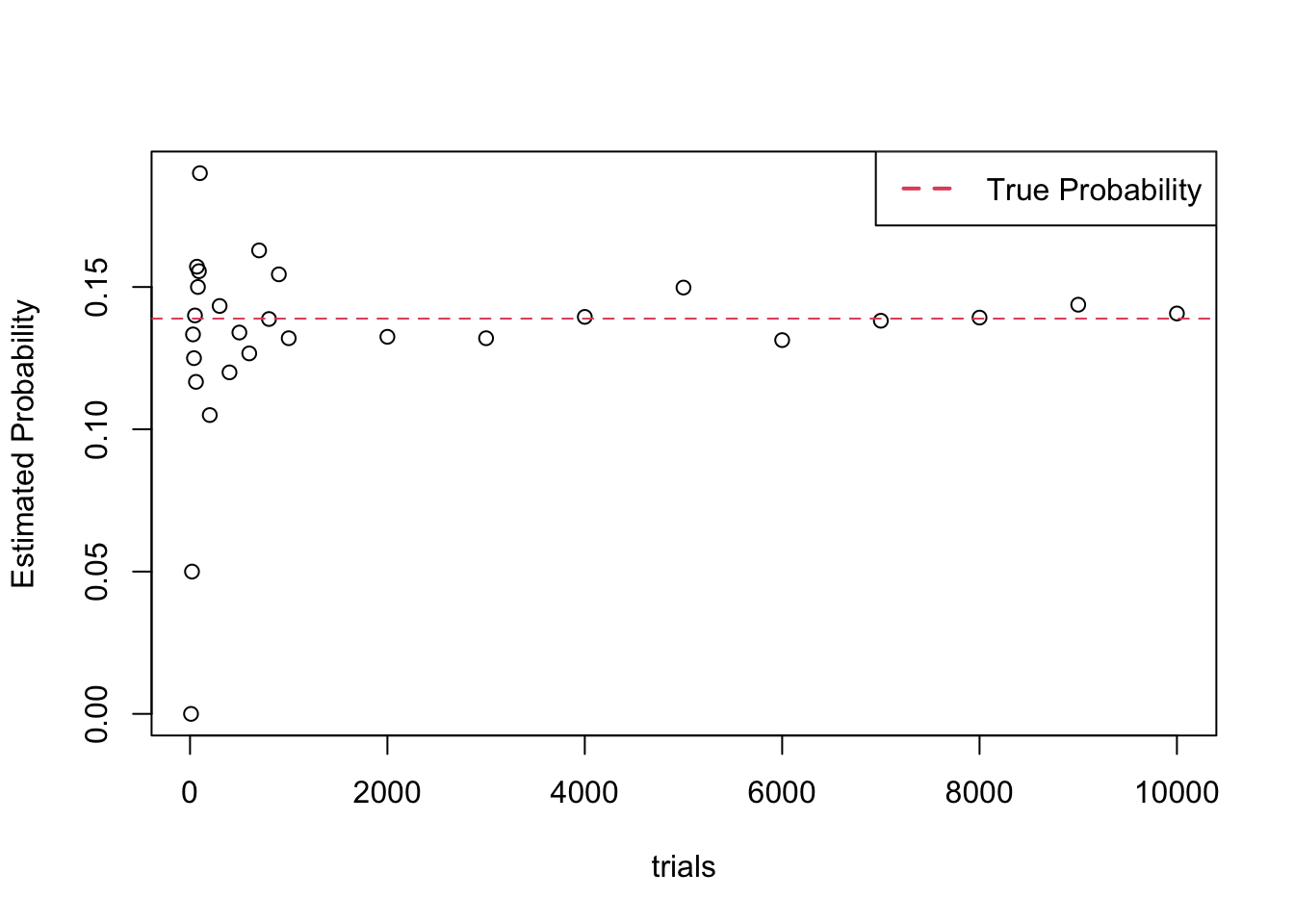
Figure 2.1: Illustration of the Law of Large Numbers. Probability estimates from simulation converge to the true probability as the number of trials increases.
The downside to using more trials is that it takes more time to do the simulation, which can become very important if each trial itself takes a considerable amount of time. As a general rule of thumb, we have found that using 10,000 trials is a good compromise between speed and accuracy.
A fair coin is repeatedly tossed.9 Estimate the probability that you observe heads for the third time on the 10th toss.
In this example, an outcome of the experiment is ten tosses of the coin. The event “you observe heads for the third time on the 10th toss” is complicated, and most of the work involves testing whether that event occurred.
As before, we build this up in stages. Begin by simulating an outcome, a sample of ten tosses of a coin:
coinToss <- sample(c("H", "T"), 10, replace = TRUE)
coinToss
## [1] "T" "T" "T" "T" "H" "T" "T" "H" "T" "T"In order for the event to occur, we need for there to be exactly three heads, so we count the number of heads and check whether it is equal to three:
sum(coinToss == "H")## [1] 2sum(coinToss == "H") == 3## [1] FALSENext, we also need to make sure that we had only two heads in the first nine tosses. So, we look only at the first nine tosses:
coinToss[1:9]## [1] "T" "T" "T" "T" "H" "T" "T" "H" "T"and add up the heads observed in the first nine tosses:
sum(coinToss[1:9] == "H") == 2## [1] TRUENote that both of those have to be true in order for the event to occur:
sum(coinToss == "H") == 3 & sum(coinToss[1:9] == "H") == 2## [1] FALSEWe put this inside replicate and compute the probability:
event <- replicate(10000, {
  coinToss <- sample(c("H", "T"), 10, replace = TRUE)
  (sum(coinToss == "H") == 3) & (sum(coinToss[1:9] == "H") == 2)
})

mean(event)
## [1] 0.0369The probability of observing heads for the third time on the 10th toss is about 3%.
The test that there were three total heads but only two on the first nine tosses is not the only way to approach this problem. Here are two other tests that give the same result by looking at the tenth coin toss:
sum(coinToss == "H") == 3 & coinToss[10] == "H"## [1] FALSEsum(coinToss[1:9] == "H") == 2 & coinToss[10] == "H"## [1] FALSEEstimate the probability that out of 25 randomly selected people, at least two will have the same birthday. Assume that all birthdays are equally likely, except that none are leap-day babies.
An outcome of this experiment is 25 randomly selected birthdays, and the event \(B\) is that at least two birthdays are the same. Simulating the experiment is straightforward, with sample:
birthdays <- sample(x = 1:365, size = 25, replace = TRUE)
birthdays
## [1] 324 167 129 299 270 187 307 85 277 362 330 263 329 79 213 37 105
## [18] 217 165 290 362 89 289 340 326Next, we test for the event \(B\). In order to do this, we need to be able to find any duplicates in a vector.
R has many, many functions that can be used with vectors. For most things that you want to do, there will be an R function that does it.
In this case it is anyDuplicated(), which returns the location of the first duplicate if there are any, and zero otherwise.
The important thing to learn here isn’t necessarily this particular function, but rather the fact that most tasks are possible via some built-in functionality.
anyDuplicated(birthdays)## [1] 21It happens that our sample did have two of the same birthday. At location 21 of the birthday vector, the number 362 appears. That same number
showed up earlier in location 10. The event \(B\) occurred in this example, and we can test for it by checking that the result of anyDuplicated is larger than 0. Putting it all together:
eventB <- replicate(n = 10000, {
  birthdays <- sample(x = 1:365, size = 25, replace = TRUE)
  anyDuplicated(birthdays) > 0
})
mean(eventB)
## [1] 0.5631The probability of this event is approximately 0.56. Interestingly, we see that it is actually quite likely that a group of 25 people will contain two with the same birthday.
Modify the above code to take into account leap years.
Three numbers are picked uniformly at random from the interval \((0,1)\). What is the probability that a triangle can be formed whose side-lengths are the three numbers that you chose?
Solution: We need to be able to simulate picking three numbers at random from the interval \((0, 1)\).
We will see later in the book that the way to do this is via runif(3, 0, 1), which returns 3 numbers randomly chosen between 0 and 1.
We then need to check whether the sum of the two smaller numbers is larger than the largest number. We use the sort command to sort the three numbers into increasing order, as follows:
event <- replicate(10000, {
  x <- sort(runif(3, 0, 1))
  sum(x[1:2]) > x[3]
})
mean(event)
## [1] 0.4979According to Rick Wicklin, 10 the proportion of M&M’s of various colors produced in the New Jersey M&M factory are as shown in Table 2.1.
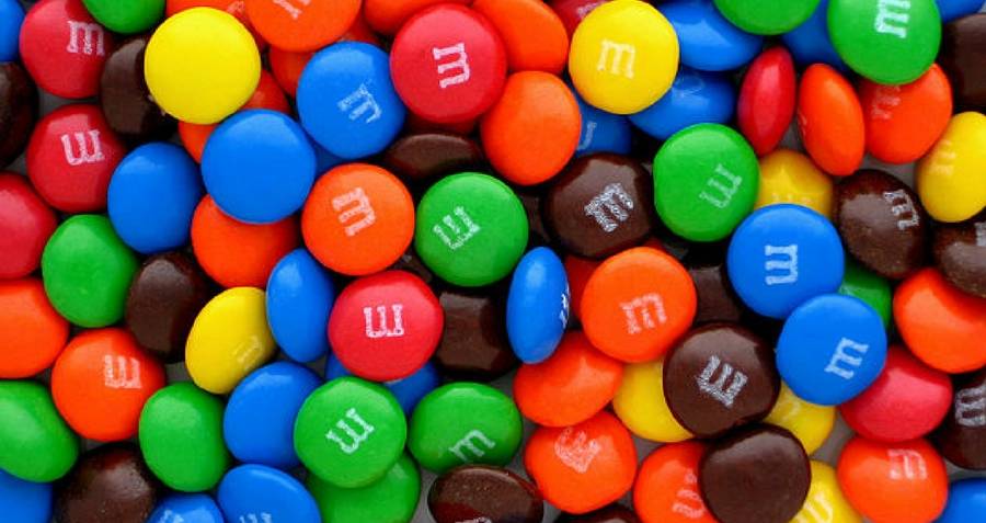
Evan Amos. Public domain https://commons.wikimedia.org/wiki/File:Plain-M&Ms-Pile.jpg
| Color | Percentage |
|---|---|
| Blue | 25.0 |
| Orange | 25.0 |
| Green | 12.5 |
| Yellow | 12.5 |
| Red | 12.5 |
| Brown | 12.5 |
If you buy a bag from the New Jersey factory that contains 35 M&M’s, what is the probability that it will contain exactly 9 Blue and 5 Red M&M’s?
To do this, we can use the prob argument in the sample function, as follows.
mm.colors <- c("Blue", "Orange", "Green", "Yellow", "Red", "Brown")
mm.probs <- c(25, 25, 12.5, 12.5, 12.5, 12.5)
bag <- sample(
  x = mm.colors,
  size = 35,
  replace = TRUE,
  prob = mm.probs
)
sum(bag == "Blue") # counts the number of Blue M&M's
## [1] 11event <- replicate(10000, {
bag <- sample(
x = mm.colors,
size = 35,
replace = TRUE,
prob = mm.probs
)
sum(bag == "Blue") == 9 & sum(bag == "Red") == 5
})
mean(event)## [1] 0.02912.3 Conditional probability and independence
Sometimes when considering multiple events, we have information that one of the events has occurred. This new information requires us to reconsider the probability that the other event occurs. For example, suppose that you roll two dice and one of them falls off of the table where you cannot see it, while the other one shows a 4. We would want to update the probabilities associated with the sum of the two dice based on this information. The new probability that the sum of the dice is 2 would be 0, the new probability that the sum of the dice is 5 would be 1/6 because that is just the probability that the die that we cannot see is a “1,” and the new probability that the sum of the dice is 7 would also be 1/6 (which is the same as its original probability).
Formally, we have the following definition.
Let \(A\) and \(B\) be events in the sample space \(S\), with \(P(B) \not= 0\). The conditional probability of \(A\) given \(B\) is \[ P(A|B) = \frac{P(A \cap B)}{P(B)} \]
We read \(P(A|B)\) as “the probability of \(A\) given \(B\).”
It is important to keep straight in your mind that the fixed idiom \(P(A|B)\) means the probability of \(A\) given \(B\), or the probability that \(A\) occurs given that \(B\) occurs. \(P(A|B)\) does not mean the probability of some event called \(A|B\).
In mathematics, the vertical bar symbol | is used for conditional probability, and you would write \(A \cup B\) for the event “\(A\) or \(B\).”
In R, the vertical bar denotes the or operator. You do not use the vertical bar in R to work with conditional probability.
The general process of assuming that \(B\) occurs and making computations under that assumption is called conditioning on \(B\). Note that in order to condition on \(B\) in the definition of \(P(A|B)\), we must assume that \(P(B)\not= 0\), since otherwise we would get \(\frac {0}{0}\), which is undefined. This also makes some intuitive sense. If we assume that a probability zero event occurs, then probability of further events conditioned on that would need to be undefined.
Two dice are rolled. What is the probability that both dice are 4, given that the sum of two dice is 8?
Solution: Let \(A\) be the event “both dice are 4” and \(B\) be the event “the sum is 8.” Then \[ P(A|B) = P(A \cap B)/P(B) = \frac{1/36}{5/36} = 1/5. \] Rolling two 4s is the hardest way to get an 8. Check that the probability of rolling one three and one five is 2/5, and also for one two and one six.
With conditional probability, the order of the two events is important. Suppose we reverse the order, and ask: “What is the probability that the sum of two dice is 8, given that both dice are 4?” Now the answer is 1, because if both dice are 4, then the sum is certainly 8. Formally, with the events defined as in Example 2.19: \[ P(B|A) = P(B \cap A)/P(A) = \frac{1/36}{1/36} = 1. \]
Two simple facts about conditional probability are:
- \(P((A \cap B)|B) = P(A|B)\).
- \(P(A \cup B|B) = 1\).
In words, statement 1 says that the probability of “\(A\) and \(B\)” given \(B\) is the probability of \(A\) given \(B\). Arguing informally, assume that we know that \(B\) occurs. Then the probability that both \(A\) and \(B\) occur is just the probability that \(A\) occurs. Using set notation:
\[\begin{align*} P((A \cap B)|B) &= P((A \cap B) \cap B)/P(B)\\ &= P(A\cap (B \cap B))/P(B)\\ &= P(A \cap B)/P(B)\\ &= P(A|B). \end{align*}\]
We included parentheses around \((A \cap B)\) above, but we did not need to. Remember, there is no event called “\(B|B\),” so the only possible interpretation of \(P(A \cap B | B)\) is \(P((A \cap B)|B)\).
Statement 2 is left as Exercise 2.24.
2.3.1 Independent events
We have seen examples where the probability of \(A\) given \(B\) can be larger than \(P(A)\), smaller than \(P(A)\), or equal to \(P(A)\). Of particular interest are pairs of events \(A\) and \(B\) such that knowledge that one of the events occurs does not impact the probability that the other event occurs.
Two events are said to be independent if knowledge that one event occurs does not give any probabilistic information as to whether the other event occurs. Formally, we say that \(A\) and \(B\) are independent if \(P(A \cap B) = P(A) P(B)\).
Events \(A\) and \(B\) are said to be dependent if they are not independent.
It is not immediately clear why the formal statement in the definition of independence implies the intuitive statement that “the knowledge that one event occurs does not give any probabilistic information as to whether the other event occurs.” To see that, we assume \(P(B) \not= 0\) and compute:
\[ P(A|B) = P(A \cap B)/P(B) = \frac{P(A)P(B)}{P(B)} = P(A) \]
If \(P(A) \not= 0\), a similar computation shows that \(P(B|A) = P(B)\) and proves the following theorem.
Let \(A\) and \(B\) be events with non-zero probability in the sample space \(S\). The following are equivalent:
- \(A\) and \(B\) are independent.
- \(P(A \cap B) = P(A)P(B)\).
- \(P(A|B) = P(A)\).
- \(P(B|A) = P(B)\).
Part 2 of Theorem 2.3 is called the multiplication rule for independent events.
Usually independence will be an assumption that we make about events and we will use that assumption to apply the multiplication rule. Here is a simple example.
You and your friend each purchase a bag of M&M’s, with colors coming from the probability distribution shown in Example 2.17. What is the probability that both of you get a blue M&M as the first candy out of your bag?
There are two events here: \(A_1\) is that your first M&M is blue, and \(A_2\) is that your friend’s first M&M is blue. It is reasonable to assume these are independent, since what color you draw from your bag should have no effect on the color of M&M your friend draws from their bag. Since both \(P(A_1) = 0.25\) and \(P(A_2) = 0.25\), the multiplication rule shows that \[ P(\text{you both get blue}) = P(A_1 \cap A_2) = P(A_1)P(A_2) = 0.25 \cdot 0.25 = 0.0625. \] There is a 6.25% chance you both get a blue M&M first.
It is important to develop an intuition about independence in order to determine whether the assumption of independence is reasonable.
Consider the following scenarios, and determine whether the events indicated are most likely dependent or independent.
- A day in the last 365 days is selected at random. Event \(A\) is that the high temperature in St. Louis, Missouri on that day was greater than 90 degrees. Event \(B\) is that the high temperature on that same day in Cape Town, South Africa was greater than 90 degrees.
- Two coins are flipped, and \(A\) is the event that the first coin lands on heads, while \(B\) is the event that the second coin lands on heads.
- Six patients are given a tuberculosis skin test, which requires a professional to estimate the size of the reaction to the tuberculin agent. Two professionals, Alexis and Angel, are randomly chosen. Let \(A\) be the event that Alexis estimates the size of the reaction in each of patients 1-5 to be larger than Angel does. Let \(B\) be the event that Alexis estimates the size of the reaction in patient 6 to be larger than Angel does.
In scenario 1, the events are dependent. If we know that the high temperature in St. Louis was greater than 90 degrees, then the day was most likely a day in June, July, August, or September, which gives us probabilistic information about whether the high temperature in Cape Town was greater than 90 degrees on that day. (In this case, it means that it was very unlikely, since that is winter in the southern hemisphere.)
In scenario 2, the events are independent, or at least approximately so. One could argue that knowing that one of the coins is heads means the person tossing the coins might be more likely to obtain heads when tossing coins. However, the potential effect here seems so weak based on experience, that it is a reasonable assumption that the events are independent.
In scenario 3, it may be inadvisable to assume that the events are independent. Of course, they may be. It could be that Alexis and Angel are well-trained, and there is no bias in their measurements. However, it is also possible that there is something systematic about how they measure the reactions so that one of them usually measures it as larger than the other one does. Knowing \(A\) may be an indication that Alexis does systematically measure reactions as larger than Angel does. (Of course, it would also be interesting to know which one was closer to the true value, but that is not what we are worried about at this point.) Later, we will develop tools that will allow us to make a more quantitative statement about this type of problem.
Two dice are rolled. It is reasonable to assume that events concerning one die are independent of events concerning the other die. For more interesting events involving both dice, we may use the definition of independence to check.
Let \(A\) be the event “the sum of the dice is 8,” let \(B\) be the event “the sum of the dice is 7,” and let \(C\) be the event “The first die is a 5.” Show that:
- \(A\) and \(B\) are dependent.
- \(A\) and \(C\) are dependent.
- \(B\) and \(C\) are independent.
For part 1, \(P(A) = 5/36\), and \(P(B) = 6/36\) but \(P(A \cap B) = 0\) since it’s not possible to roll an 8 and a 7 at the same time (\(A\) and \(B\) are disjoint). Since \(P(A)P(B) \neq P(A \cap B)\) the events are dependent.
For part 2, \(P(A) = 5/36\) and \(P(A|C) = 1/6\) since given a 5 on the first die, there is a 1/6 chance of rolling a 3 on the second to make a sum of 8. Since \(P(A) \neq P(A|C)\), the events \(A\) and \(C\) are not independent.
Finally, \(P(B) = 6/36 = 1/6\) and \(P(B|C) = 1/6\). Therefore, \(B\) and \(C\) are independent. You might expect that knowing one die tells you something about the sum, as it does in part 2. However, a roll of 7 is special. It happens 1/6 of the time, and if you know the value of one die there is still a 1/6 chance the second die will be the one number needed to make 7.
We now extend the definition of independence to mutual independence of multiple events. The intuition remains the same: mutual independence means that knowing something about some of these events gives no probabilistic information about the others. However, the notion of mutual independence is stronger than just saying that every pair of the events are independent – see Exercise 2.25. We require a multiplication rule for every pair, triple, and so on for every sub-collection of these events.
A collection of events \(A_1, A_2, \dotsc, A_n \subset S\) are mutually independent if for any sub-collection \(A_{i_1}, \dotsc, A_{i_k}\) we have \[ P(A_{i_1} \cap A_{i_2} \cap \dotsb \cap A_{i_k}) = P(A_{i_1}) \cdot P(A_{i_2}) \cdot \ldots \cdot P(A_{i_k}) \]
In this book, we will use Definition 2.24 exclusively as a multiplication rule, where events \(A_1, \dotsc, A_n\) are assumed to be independent and we apply \(P(A_1 \cap \dotsb \cap A_n) = P(A_1) \cdot \ldots \cdot P(A_n)\).
Suppose you roll five ordinary dice. What is the probability that all of them show six?
Let event \(D_i\) be the event that the \(i^\text{th}\) die shows six. We don’t expect the dice to affect each other, so the events \(D_1, \dotsc, D_5\) are mutually independent. Then
\[\begin{align*} P(\text{all sixes}) &= P(D_1 \cap D_2 \cap D_3 \cap D_4 \cap D_5) = \\ & P(D_1) \cdot P(D_2) \cdot P(D_3) \cdot P(D_4) \cdot P(D_5) = \left(\frac{1}{6}\right)^5 \approx 0.000129. \end{align*}\]
In the next example, we illustrate a method to compute probabilities involving the idea of “at least one” or “any.”
The trick is to convert logical OR into logical AND using DeMorgan’s Law.
Example 2.26 also illustrates the use of the
any command in R, which takes a T/F vector and detects if any entry is TRUE.
Suppose you roll five ordinary dice. What is the probability that at least one six appears?
Let \(A\) be the event “at least one six appears.” Let \(D_i\) be the event that the \(i^{\text{th}}\) die is a six. Then \(A = D_1 \cup D_2 \cup D_3 \cup D_4 \cup D_5\). Since the \(D_i\) are not disjoint, we cannot use the addition rule for disjoint events. However, the \(D_i\) events are independent. Observe that “not \(A\)” is the event “no sixes appear,” so that \[ \text{not } A = (\text{not } D_1) \text{ AND } (\text{not } D_2) \text{ AND } \dotsc \text{ AND } (\text{not } D_5) \] Using the multiplication rule for independent events
\[ P(\text{not } A) = P(\text{not } D_1) \cdot P(\text{not } D_2) \cdot \dotsc \cdot P(\text{not } D_5) = (5/6)^5\]
Finally, \(P(A) = 1 - P(\text{not } A) = 1 - (5/6)^5 \approx 0.598\).
To do this with simulation:
mean(replicate(10000, {
  roll5 <- sample(1:6, 5, replace = TRUE)
  any(roll5 == 6)
}))
## [1] 0.59672.3.2 Simulating conditional probability
Simulating conditional probabilities is challenging. In order to estimate \(P(A|B)\), we will estimate \(P(A \cap B)\) and \(P(B)\) and then divide the two answers. This is not the most efficient or best way to estimate \(P(A|B)\), but it is easy to do with the tools that we already have developed.
Two dice are rolled. Estimate the conditional probability that the sum of the dice is at least 10, given that at least one of the dice is a 6.
First, we estimate the probability that the sum of the dice is at least 10 and at least one of the dice is a 6.
eventAB <- replicate(10000, {
  dieRoll <- sample(1:6, 2, replace = TRUE)
  (sum(dieRoll) >= 10) && (6 %in% dieRoll)
})
probAB <- mean(eventAB)
Next, we estimate the probability that at least one of the dice is a 6.
eventB <- replicate(10000, {
  die_roll <- sample(1:6, 2, replace = TRUE)
  6 %in% die_roll
})
probB <- mean(eventB)
Finally, we take the quotient.
probAB / probB## [1] 0.4560601The correct answer is \(P(A\cap B)/P(B) = \frac{5/36}{11/36} = 5/11 \approx 0.4545\).
2.3.3 Bayes’ Rule and conditioning
The Law of Total Probability allows the computation of the probability of an event by “conditioning” on another event.
Let \(A\) and \(B\) be events in the sample space \(S\). Then \[ P(A) = P(A \cap B) + P(A \cap \overline{B}) = P(A|B)P(B) + P(A|\overline{B})P(\overline{B}) \]
This formula breaks the probability of \(A\) into two pieces, one where \(B\) happens and one where \(B\) does not happen.
Since the sample space \(S = B \cup \overline{B}\), \(A = A \cap S = (A \cap B) \cup (A \cap \overline{B})\). Because \(A \cap B\) and \(A \cap \overline{B}\) are disjoint, \[ P(A) = P\left((A \cap B) \cup (A \cap \overline{B})\right) = P(A \cap B) + P(A \cap \overline{B}). \] The second equality follows from Definition 2.18, the definition of conditional probability.
The name “Mary” was given to 7065 girls in 1880, and to 11475 girls in 1980. There were 97583 girls born in 1880, and 177907 girls born in 1980. Suppose that a randomly selected girl born in 1880 or 1980 is chosen. What is the probability that the girl’s name is “Mary”?
To solve this, let’s let \(A\) be the event that the randomly selected girl’s name is Mary. If we knew what year the girl was born in, then we would have a good idea what to do. We don’t, so we condition on the birth year. Let \(B\) be the event that the randomly selected girl was born in 1880.
Applying the Law of Total Probability, \[\begin{align*} P(A) &= P(A|B)P(B) + P(A|\overline{B})P(\overline{B}) \\ &= \frac{7065}{97583} \frac{97583}{97583 + 177907} + \frac{11475}{177907} \frac{177907}{97583 + 177907}\\ &= 0.0676 \end{align*}\]
The probability that the randomly selected girl’s name is Mary is 0.0676.
Bayes’ Rule is a simple statement about conditional probabilities that allows the computation of \(P(A|B)\) from \(P(A)\).
Let \(A\) and \(B\) be events in the sample space \(S\). \[ P(A|B) = \frac{P(B|A)P(A)}{P(B)} = \frac{P(B|A)P(A)}{P(B|A)P(A) + P(B|\overline{A})P(\overline{A})} \]
From the definition of conditional probability (Definition 2.18), \(P(A\cap B) = P(A|B)P(B)\). Switching \(A\) and \(B\) gives \(P(B \cap A) = P(B|A)P(A)\). Since \(A\cap B = B\cap A\), we have \(P(A|B)P(B) = P(B|A)P(A)\). Dividing both sides by \(P(B)\) proves the first equality. The second equality is simply the Law of Total Probability applied to \(P(B)\) in the denominator.
Using the evidential interpretation of probability, Bayes’ Rule forms the foundation of Bayesian statistics. Suppose we have some prior evidence about the event \(A\), in the form of \(P(A)\). Then \(P(A|B)\) is the knowledge we have about \(A\) after accounting for the information that \(B\) is true. With this interpretation, the rule is a way to update our evidence for \(A\) given new information.
In a certain hotel near the US/Canada border, 70% of hotel guests are American and 30% are Canadian. It is known that 40% of Americans wear white socks, while 20% of Canadians wear white socks. Suppose you randomly select a person and observe that they are wearing white socks. What is the probability that the person is Canadian?
Let \(A\) be the event that a randomly person selected is Canadian. We are given that \(P(A) = 0.3\) as prior knowledge. Let \(B\) denote the event that a randomly selected person is wearing white socks. We are asked to find \(P(A|B)\), the probability that a randomly selected person is Canadian, given that they are wearing white socks. Since relatively few Canadians wear white socks, \(P(A|B)\) should be lower than 0.3. Bayes’ Rule computes the probability exactly:
\[\begin{align*} P(A|B) &= \frac{P(B|A)P(A)}{P(B|A)P(A) + P(B|\overline{A})P(\overline{A})}\\ &= \frac{0.2 \times 0.3}{0.2 \times 0.3 + 0.4 \times 0.7} = 0.176 \end{align*}\]
Now that we know the person is wearing white socks, there is only a 0.176 probability they are Canadian.
There is a more general version of the Law of Total Probability and Bayes’ Rule.
We say that \(A_1, \ldots, A_k\) is a partition of the sample space \(S\) if \(\cup_{i = 1}^k A_i = S\) and \(A_i \cap A_j = \emptyset\) whenever \(i \not= j\).
Let \(A_1, \ldots, A_k\) be a partition of the sample space \(S\) and let \(B\) be an event. Then, \[ P(B) = \sum_{i = 1}^k P(B \cap A_i) = \sum_{i = 1}^k P(B|A_i)P(A_i) \] and \[ P(A_j|B) = \frac{P(B|A_j)P(A_j)}{\sum_{i = 1}^k P(B|A_i)P(A_i)} \]
Exercise 2.32 requires this more general form.
2.4 Counting arguments
Given a sample space \(S\) consisting of equally likely simple events, and an event \(E\), recall that \(P(E) = \frac{|E|}{|S|}\). For this reason, it can be useful to be able to carefully enumerate the elements in a set. While an interesting topic, this is not a point of emphasis of this book, as (1) we assume that students have seen some basic counting arguments in the past and (2) we emphasize simulation techniques.
This text will only work with two counting rules:
If there are \(m\) ways to do something, and for each of those \(m\) ways there are \(n\) ways to do another thing, then there are \(m \times n\) ways to do both things.
The number of ways of choosing \(k\) distinct objects from a set of \(n\) is given by \[ {\binom{n}{k}} = \frac{n!}{k!(n - k)!} \]
The R command for computing \({\binom{n}{k}}\) is choose(n,k).
A coin is tossed 10 times. Some possible outcomes are HHHHHHHHHH, HTHTHTHTHT, and HHTHTTHTTT. Since each toss has two possibilities, the rule of product says that there are \(2\cdot 2\cdot 2\cdot 2\cdot 2\cdot 2\cdot 2\cdot 2\cdot 2\cdot 2 = 2^{10} = 1024\) possible outcomes for the experiment. We expect each possible outcome to be equally likely, so the probability of any single outcome is 1/1024.
Let \(E\) be the event “we flipped exactly three heads.” This might happen as the sequence HHHTTTTTTT, or TTTHTHTTHT, or many other ways. What is \(P(E)\)? To compute the probability, we need to count the number of possible ways that three heads may appear. Since the three heads may appear in any of the ten slots, the answer is
\[ |E| = {\binom{10}{3}} = \frac{10 \times 9 \times 8}{3 \times 2 \times 1} = 120. \]
Then \(P(E) = 120/1024 \approx 0.117\). We can also estimate \(P(E)\) with simulation:
event <- replicate(10000, {
  flips <- sample(c("H", "T"), 10, replace = TRUE)
  heads <- sum(flips == "H")
  heads == 3
})
mean(event)
## [1] 0.1211Suppose that in a class of 10 boys and 10 girls, 5 students are randomly chosen to present work at the board.
- What is the probability that all 5 students are boys?
- What is the probability that exactly 4 of the students are girls?
Let \(E\) be the event “all 5 students are boys.” The sample space consists of all ways of choosing 5 students from a class of 20, so choose(20,5) = 15504. The event \(E\) consists of all ways of choosing 5 boys from a group of 10, so choose(10, 5) = 252. Therefore, the probability is 252/15504 = .016.
Next, let \(A\) be the event “exactly 4 of the students are girls.” The sample space is still the same. The event \(A\) can be broken down into two tasks: choose the 4 girls and choose the 1 boy. By the multiplication principle, there are choose(10, 4) * choose(10,1) = 2100 ways of doing that. Therefore, the probability is 2100/15504 = .135.
A deck of 52 cards has four suits11 and 13 ranks in each suit: 2,3,4,5,6,7,8,9,10,J,Q,K,A. If you are dealt two cards, what is the probability they have the same rank?
The sample space is all possible two card hands. Since there are 52 cards in the deck, there are \(\binom{52}{2} = 1326\) possible hands.
The event “both cards have the same rank” can be broken down into two choices. First, choose the rank those cards will have. There are 13 choices. Next choose two of the four cards with that rank for your hand, for which there are \(\binom{4}{2} = 6\) choices. Then there are \(13 \times 6 = 78\) ways for your hand to have a pair of the same rank.
The probability of getting a pair is \(78/1326 \approx 0.059\).
To estimate with simulation, we build a deck of cards by thinking of the ranks as the numbers 2 through 14 and then using ‘rep’ to produce four copies:
deck <- rep(2:14, 4)
pair <- replicate(10000, {
  hand <- sample(deck, 2)
  hand[1] == hand[2]
})
mean(pair)
## [1] 0.059Vignette: Negative surveys
Suppose you are trying to get information about a relatively sensitive topic on a survey. For example, you might want to determine how much money people owe on their credit cards at a given moment in time. While this information is not terribly sensitive, it is sensitive enough that some people might not feel comfortable telling the truth in a survey.
One way to combat this problem is with a negative survey.12 Instead of asking the participant to answer the question correctly, you ask the participant to select one of the answers that is not true according to some probability distribution. As an example, we could ask the following:
How much money do you not owe on your credit cards as of today?
- Zero dollars.
- Between 1 and 1000 dollars.
- More than 1000 dollars.
We instruct the respondent to randomly select one of the answers that is not correct. In practice, we might want to have more possible answers; we are using three answers to illustrate the mathematics behind the scenes.
Suppose you collect 1000 surveys, and your proportion of answers are:
- 50%
- 30%
- 20%
Now you want to figure out the percentages of people who owe certain values, rather than what they do not owe. We use 0.5, 0.3, and 0.2 as our estimates for the true proportion of people who will answer a, b, and c, respectively, when given this survey. Let \(A\) be the event that a person owes zero dollars, \(B\) be the event they owe between 1 and 1000 dollars, and \(C\) be the event that they owe more than 1000 dollars. Let \(D\) be the event they select choice a on the survey, \(E\) be the event they select choice b on the survey, and \(F\) be the event they select choice c on the survey. By Theorem 2.4, the Law of Total Probability,
\[ \begin{pmatrix} P(D) &=& ~~~~0 \times P(A) &+ &1/2 \times P(B) &+ &1/2 \times P(C) \\ P(E) &=& 1/2 \times P(A) &+ & ~~~~0 \times P(B) &+ &1/2 \times P(C) \\ P(F) &=& 1/2 \times P(A) &+&1/2 \times P(B) &+& ~~~~0 \times P(C) \end{pmatrix} \]
Using some matrix algebra,
\[ \begin{pmatrix} 0.5\\0.3\\0.2 \end{pmatrix} = \begin{pmatrix} 0&1/2&1/2\\1/2&0&1/2\\1/2&1/2&0 \end{pmatrix} \begin{pmatrix} P(A)\\P(B)\\P(C)\end{pmatrix} \]
Now multiply both sides by the inverse of the square matrix in the above equation to get
\[ \begin{pmatrix} 0&1/2&1/2\\1/2&0&1/2\\1/2&1/2&0 \end{pmatrix} ^{-1} \begin{pmatrix} 0.5\\0.3\\0.2 \end{pmatrix} = \begin{pmatrix} P(A)\\P(B)\\P(C)\end{pmatrix} \]
Using R, we have
solve(matrix(c(0, 1, 1, 1, 0, 1, 1, 1, 0),
  byrow = TRUE,
  ncol = 3
) * 1 / 2) %*%
  matrix(c(.5, .3, .2), ncol = 1)
## [,1]
## [1,] 0.0
## [2,] 0.4
## [3,] 0.6We see that 0% of the people owe zero dollars, 40% owe between 1 and 1000 dollars, and 60% owe more than 1000 dollars.
Exercises
Exercises 2.1 – 2.3 require material through Section 2.1.
When rolling two dice, what is the probability that one die is twice the other?
Consider an experiment where you roll two dice, and subtract the smaller value from the larger value (getting 0 in case of a tie).
- What is the probability of getting 0?
- What is the probability of getting 4?
A hat contains slips of paper numbered 1 through 6. You draw two slips of paper at random from the hat, without replacing the first slip into the hat.
- Write out the sample space \(S\) for this experiment.
- Write out the event \(E\), “the sum of the numbers on the slips of paper is 4.”
- Find \(P(E)\).
- Let \(F\) be the event “the larger number minus the smaller number is 0.” What is \(P(F)\)?
Exercises 2.4 – 2.19 require material through Section 2.2.
Suppose there are two boxes and each contain slips of papers numbered 1-8. You draw one number at random from each box.
- Estimate the probability that the sum of the numbers is 8.
- Estimate the probability that at least one of the numbers is a 2.
Suppose the proportion of M&M’s by color is:
\[ \begin{array}{cccccc} Yellow & Red & Orange & Brown & Green & Blue \\ 0.14 & 0.13 & 0.20 & 0.12 & 0.20 & 0.21 \end{array} \]
- What is the probability that a randomly selected M&M is not green?
- What is the probability that a randomly selected M&M is red, orange, or yellow?
- Estimate the probability that a random selection of four M&M’s will contain a blue one.
- Estimate the probability that a random selection of six M&M’s will contain all six colors.
With the distribution from Problem 2.5, suppose you buy a bag of M&M’s with 30 pieces in it. Estimate the probability of obtaining at least 9 Blue M&M’s and at least 6 Orange M&M’s in the bag.
Blood types O, A, B, and AB have the following distribution in the United States: \[ \begin{array}{lcccc} \text{Type} &A& AB & B & O\\ \text{Probability} & 0.40 & 0.04 & 0.11 & 0.45 \end{array} \] What is the probability that two randomly selected people have the same blood type?
Use simulation to estimate the probability that a 10 is obtained when two dice are rolled.
Estimate the probability that exactly 3 heads are obtained when 7 coins are tossed.
Estimate the probability that the sum of five dice is between 15 and 20, inclusive.
Suppose a die is tossed repeatedly, and the cumulative sum of all tosses seen is maintained. Estimate the probability that the cumulative sum ever is exactly 20.
(Hint: the function cumsum computes the cumulative sums of a vector.)
- Simulate rolling two dice and adding their values. Perform 10,000 simulations and make a bar chart showing how many of each outcome occurred.
- You can buy trick dice, which look (sort of) like normal dice. One die has numbers 5, 5, 5, 5, 5, 5. The other has numbers 2, 2, 2, 6, 6, 6. Simulate rolling the two trick dice and adding their values. Perform 10,000 simulations and make a bar chart showing how many of each outcome occurred.
- Sicherman dice also look like normal dice, but have unusual numbers. One die has numbers 1, 2, 2, 3, 3, 4. The other has numbers 1, 3, 4, 5, 6, 8. Simulate rolling the two Sicherman dice and adding their values. Perform 10,000 simulations and make a bar chart showing how many of each outcome occurred. How does your answer compare to part (a)?
In a room of 200 people (including you), estimate the probability that at least one other person will be born on the same day as you.
In a room of 100 people, estimate the probability that at least two people were not only born on the same day, but also during the same hour of the same day. (For example, both were born between 2 and 3.)
Assuming that there are no leap-day babies and that all birthdays are equally likely, estimate the probability that at least three people have the same birthday in a group of 50 people. (Hint: try using table.)
If 100 balls are randomly placed into 20 urns, estimate the probability that at least one of the urns is empty.
A standard deck of cards has 52 cards, four each of 2,3,4,5,6,7,8,9,10,J,Q,K,A. In blackjack, a player gets two cards and adds their values. Cards count as their usual numbers, except Aces are 11 (or 1), while K, Q, J are all 10.
- “Blackjack” means getting an Ace and a value 10 card. What is the probability of getting a blackjack?
- What is the probability of getting 19? (The probability that the sum of your cards is 19, using Ace as 11)
Use R to simulate dealing two cards, and compute these probabilities experimentally.
Deathrolling in World of Warcraft works as follows. Player 1 tosses a 1000-sided die. Say they get \(x_1\). Then player 2 tosses a die with \(x_1\) sides on it. Say they get \(x_2\). Player 1 tosses a die with \(x_2\) sides on it. This pattern continues until a player rolls a 1. The player who loses is the player who rolls a 1. Estimate via simulation the probability that a 1 will be rolled on the 4th roll in deathroll.
In the game of Scrabble, players make words using letter tiles.
The data set fosdata::scrabble contains all 100 tiles.
Players begin the game by drawing seven tiles from a bag of 100 tiles. Estimate the probability that a player’s first seven tiles contain no vowels. (Vowels are A, E, I, O, and U.)
Exercises 2.20 – 2.32 require material through Section 2.3.
Two dice are rolled.
- What is the probability that the sum of the numbers is exactly 10?
- What is the probability that the sum of the numbers is at least 10?
- What is the probability that the sum of the numbers is exactly 10, given that it is at least 10?
A hat contains six slips of paper with the numbers 1 through 6 written on them. Two slips of paper are drawn from the hat (without replacing), and the sum of the numbers is computed.
- What is the probability that the sum of the numbers is exactly 10?
- What is the probability that the sum of the numbers is at least 10?
- What is the probability that the sum of the numbers is exactly 10, given that it is at least 10?
Roll two dice, one white and one red. Consider these events:
- \(A\): The sum is 7.
- \(B\): The white die is odd.
- \(C\): The red die has a larger number showing than the white.
- \(D\): The dice match (doubles).
- Which pair(s) of events are disjoint (events \(A\) and \(B\) are disjoint if \(A \cap B = \emptyset\))?
- Which pair(s) are independent?
- Which pair(s) are neither disjoint nor independent?
Suppose you do an experiment where you select ten people at random and ask their birthdays.
Here are three events:
- \(A\) : all ten people were born in February.
- \(B\) : the first person was born in February.
- \(C\) : the second person was born in January.
- Which pair(s) of these events are disjoint, if any?
- Which pair(s) of these events are independent, if any?
- What is \(P(B | A)\)?
Let \(A\) and \(B\) be events. Show that \(P(A \cup B|B) = 1\).
In an experiment where you toss a fair coin twice, define events:
- \(A\) : the first toss is heads.
- \(B\) : the second toss is heads.
- \(C\) : both tosses are the same.
Show that \(A\) and \(B\) are independent. Show that \(A\) and \(C\) are independent. Show that \(B\) and \(C\) are independent. Finally, show that \(A\), \(B\), and \(C\) are not mutually independent.
Suppose a die is tossed three times. Let \(A\) be the event “the first toss is a 5.” Let \(B\) be the event “the first toss is the largest number rolled” (the “largest” can be a tie). Determine, via simulation or otherwise, whether \(A\) and \(B\) are independent.
Suppose you have two coins that land with heads facing up with common probability \(p\), where \(0 < p < 1\). One coin is red and the other is white. You toss both coins. Find the probability that the red coin is heads, given that the red coin and the white coin are different. Your answer will be in terms of \(p\).
Bob Ross was a painter with a PBS television show, “The Joy of Painting,” that ran for 11 years.
- 91% of Bob’s paintings contain a tree13 and 85% contain two or more trees. What is the probability that he painted a second tree, given that he painted a tree?
- 18% of Bob’s paintings contain a cabin. Given that he painted a cabin, there is a 35% chance the cabin is on a lake. What is the probability that a Bob Ross painting contains both a cabin and a lake?
Ultimate frisbee players are so poor they don’t own coins. So, team captains decide which team will play offense first by flipping frisbees before the start of the game. Rather than flip one frisbee and call a side, each team captain flips a frisbee and one captain calls whether the two frisbees will land on the same side, or on different sides. Presumably, they do this instead of just flipping one frisbee because a frisbee is not obviously a fair coin - the probability of one side seems likely to be different from the probability of the other side.
- Suppose you flip two fair coins. What is the probability they show different sides?
- Suppose two captains flip frisbees. Assume the probability that a frisbee lands convex side up is \(p\). Compute the probability (in terms of \(p\)) that the two frisbees match.
- Make a graph of the probability of a match in terms of \(p\).
- One Reddit user flipped a frisbee 800 times and found that in practice, the convex side lands up 45% of the time. When captains flip, what is the probability of “same”? What is the probability of “different”?
- What advice would you give to an ultimate frisbee team captain?
- Is the two-frisbee flip better than a single-frisbee flip for deciding the offense?
Suppose there is a new test that detects whether people have a disease. If a person has the disease, then the test correctly identifies that person as being sick 99.9% of the time (the sensitivity of the test). If a person does not have the disease, then the test correctly identifies the person as being well 97% of the time (the specificity of the test). Suppose that 2% of the population has the disease. Find the probability that a randomly selected person has the disease given that they test positive for the disease.
Suppose that there are two boxes containing marbles.
Box 1 contains 3 red and 4 blue marbles. Box 2 contains 2 red and 5 blue marbles. A single die is tossed, and if the result is 1 or 2, then a marble is drawn from box 1. Otherwise, a marble is drawn from box 2.
- What is the probability that the marble drawn is red?
- What is the probability that the marble came from box 1 given that the marble is red?
Suppose that you have 10 boxes, numbered 0-9. Box \(i\) contains \(i\) red marbles and \(9 - i\) blue marbles.
You perform the following experiment. Pick a box at random, draw a marble and record its color. Replace the marble back in the box, and draw another marble from the same box and record its color. Replace the marble back in the box, and draw another marble from the same box and record its color. So, all three marbles are drawn from the same box.
- If you draw three consecutive red marbles, what is the probability that a fourth marble drawn from the same box will also be red?
- If you draw three consecutive red marbles, what is the probability that you chose box 9?
Exercises 2.33 – 2.36 require material through Section 2.4.
How many ways are there of getting 4 heads when tossing 10 coins?
How many ways are there of getting 4 heads when tossing 10 coins, assuming that the 4th head came on the 10th toss?
Six standard six-sided dice are rolled.
- How many outcomes are there?
- How many outcomes are there such that all of the dice are different numbers?
- What is the probability that you obtain six different numbers when you roll six dice?
A box contains 5 red marbles and 5 blue marbles. Six marbles are drawn without replacement.
- How many ways are there of drawing the 6 marbles? Assume that getting all 5 red marbles and the first blue marble is different than getting all 5 red marbles and the second blue marble, for example.
- How many ways are there of drawing 4 red marbles and 2 blue marbles?
- What is the probability of drawing 4 red marbles and 2 blue marbles?
All dice in this book will be assumed to be fair dice unless otherwise stated. That is, the probability of each die landing on a face is one over the number of faces, and the results of some dice do not affect the results of the other dice.↩︎
All coins in this book, unless otherwise stated, will be fair coins in the sense that the probability of heads is \(1/2\) and successive trials are independent.↩︎
C Purtill, “A Statistician Got Curious about M&M Colors and Went on an Endearingly Geeky Quest for Answers,” Quartz, March 15, 2017, https://qz.com/918008/the-color-distribution-of-mms-as-determined-by-a-phd-in-statistics/.↩︎
The names of the suits depend on the country of origin. French-suited cards are the ones most commonly used, and have Hearts, Diamonds or Tiles, Clovers or Clubs, and Pikes or Spades. German-suited cards consist of Hearts, Bells, Acorns, and Leaves, while Italian-suited cards consist of Swords, Cups, Coins, and Batons.↩︎
F Esponda and Víctor M Guerrero, “Surveys with Negative Questions for Sensitive Items,” Statistics & Probability Letters 79 (2009): 2456–61.↩︎
W Hickey, “A Statistical Analysis of the Work of Bob Ross,” FiveThirtyEight, April 14, 2014, https://fivethirtyeight.com/features/a-statistical-analysis-of-the-work-of-bob-ross/.↩︎