Probability, Statistics, and Data: A Fresh Approach Using R

Chapter 9 Rank Based Tests

In a 2013 paper, D.K. Milton et al.⁶⁸ studied the impact of wearing a surgical facemask on exhaled aerosol droplets for patients with influenza. Each subject performed two 30-minute trials, exhaling into a collection device (Figure 9.1). The subjects were tested once while wearing a facemask and once without, and the researchers counted the number of copies of the influenza virus in their fine particle droplets.

Figure 9.1: Inlet cone for the human exhaled breath air sampler used to measure influenza virus, from Milton et al.

Image credit: Milton et al.Image Credit
Milton et al. This is an open-access article distributed under the terms of the Creative Commons Attribution License. https://www.ncbi.nlm.nih.gov/pmc/articles/PMC3591312/figure/ppat-1003205-g002/

Virus counts are in the variables mask_fine and no_mask_fine within the data set fosdata::masks. The difference no_mask_fine - mask_fine will be positive if the subject exhaled less influenza virus while wearing a mask.

masks <- fosdata::masks %>%
  mutate(virus_difference = no_mask_fine - mask_fine)
summary(masks$virus_difference)

##    Min. 1st Qu.  Median    Mean 3rd Qu.    Max. 
##    -531       2      75    3809     417  102348

The virus_difference variable has two large positive outliers (26422 and 102348) that make visualization challenging. Figure 9.2 shows a dotplot⁶⁹ of the variable with those two values removed.

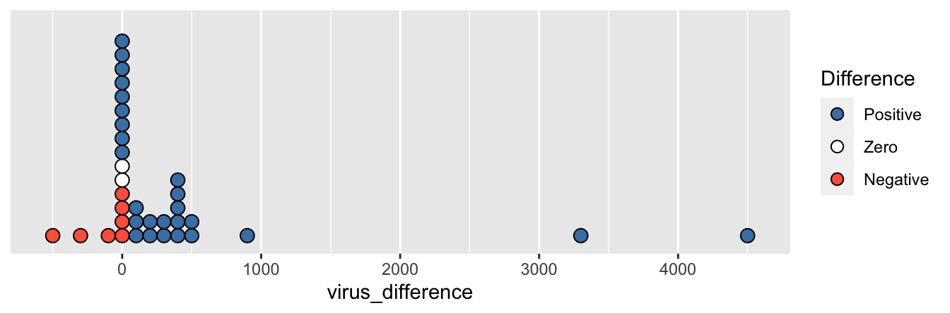
Figure 9.2: Each dot represents one patient and gives the difference in fine particle virus count between their masked and maskless trials. A positive value means the exhaled virus count was larger when not wearing a mask. Two large positive points are omitted.

Even without the largest values, it is obvious from the plot that most patients shed fewer virus particles while wearing a mask. The seven patients who shed more particles while wearing a mask had smaller differences in viral count than the 28 who shed fewer particles while wearing a mask. However, the presence of outliers (the two shown in the figure and the two even larger ones not shown) renders the \(t\)-test powerless to detect a difference between masked and unmasked patients. A paired two-sample \(t\)-test on this data results in a \(p\)-value of 0.19, not significant.

Wilcoxon rank based tests take the data and sort it from smallest to largest, replacing the actual measurements with their ranks. In this example, the ranks range from 1 to 37, for the 37 subjects of the study. Using ranks instead of the actual data values makes the test resistant to outliers while still accounting for the preponderance of positive values and the fact that those values tend to be larger.

wilcox.test(masks$mask_fine, masks$no_mask_fine, paired = TRUE)

## 
##  Wilcoxon signed rank test with continuity correction
## 
## data:  masks$mask_fine and masks$no_mask_fine
## V = 88.5, p-value = 0.000214
## alternative hypothesis: true location shift is not equal to 0

We interpret this result as saying that the median difference in viral count is positive, with \(p = 0.0002\). The low \(p\)-value suggests that masks reduce exhaled viral particles.

In this chapter we discuss rank based tests that can be used, and are still effective, on a population with outliers. Rank based tests may also be used when the measured quantity is ordinal rather than numeric.

9.1 One sample Wilcoxon signed rank test

The Wilcoxon signed rank test tests \(H_0: m = m_0\) versus \(H_a: m\not= m_0\), where \(m\) is the median of the underlying population. We will assume that the data is centered symmetrically around the median (so that the median is also the mean). There can be outliers, bimodality or any kind of tails.

Let’s look at how the test works by hand by examining a simple, made up data set. Suppose you wish to test

\[ H_0: m = 6 \qquad {\rm vs} \qquad H_a: m\not=6 \] You collect the data \(x_1 = 15, x_2 = 7, x_3 = 3, x_4 = 10\) and \(x_5 = 13\). The test works as follows:

1. Compute \(y_i = x_i - m_0\) for each \(i\). Here \(m_0 = 6\) and we get \(y_1 = 9, y_2 = 1, y_3 = -3, y_4 = 4\) and \(y_5 = 7\).
2. Let \(R_i\) be the rank of the absolute value of \(y_i\). That is, \(R_1 = 5, R_2 = 1, R_3 = 2, R_4 = 3, R_5 = 4\) since \(|y_1|\) is largest, \(|y_2|\) is smallest, etc.
3. Let \(r_i\) be the signed rank of \(R_i\); i.e., \(r_i = R_i \times {\rm sign} (y_i)\), so \(r_1 = 5, r_2 = 1, r_3 = -2, r_4 = 3, r_5 = 4\).
4. Add all of the positive ranks. We get \(r_1 + r_2 + r_4 + r_5 = 13\). That is the test statistic for this test, and it is traditionally called \(V\).
5. Compute the \(p\)-value for the test, which is the probability that we get a test statistic \(V\) which is this, or more, extreme relative to the expected value under the assumption of \(H_0\).

In order to perform the last step, we need to understand the sampling distribution of \(V\), under the assumption of the null hypothesis, \(H_0\). The ranks of our five data points will always be the numbers 1, 2, 3, 4, and 5. When \(H_0\) is true, each data point is equally likely to be positive or negative, and its corresponding rank will be included in the sum in item 4 above half of the time. So, the expected value is \[ E(V) = \frac{1}{2}\cdot 1 + \frac{1}{2}\cdot 2 + \frac{1}{2}\cdot 3 + \frac{1}{2}\cdot 4 + \frac{1}{2}\cdot5 = \frac{15}{2} = 7.5 \] In our example, \(V = 13\), which is 5.5 away from the expected value of 7.5.

For the probability distribution of \(V\), Table 9.1 lists all \(2^5 = 32\) possibilities of how the ranks could be signed. Since we have assumed that the distribution is centered about its mean, each of the possibilities is equally likely. Therefore, we can compute the proportion of rows in the table that lead to a test statistic at least 5.5 away from the expected value of 7.5.

Table 9.1: All possible sums of positive signed ranks.

r1	r2	r3	r4	r5	Sum of positive ranks	Far from 7.5?
-1	-2	-3	-4	-5	0	Yes
-1	-2	-3	-4	5	5
-1	-2	-3	4	-5	4
-1	-2	-3	4	5	9
-1	-2	3	-4	-5	3
-1	-2	3	-4	5	8
-1	-2	3	4	-5	7
-1	-2	3	4	5	12
-1	2	-3	-4	-5	2	Yes
-1	2	-3	-4	5	7
-1	2	-3	4	-5	6
-1	2	-3	4	5	11
-1	2	3	-4	-5	5
-1	2	3	-4	5	10
-1	2	3	4	-5	9
-1	2	3	4	5	14	Yes
1	-2	-3	-4	-5	1	Yes
1	-2	-3	-4	5	6
1	-2	-3	4	-5	5
1	-2	-3	4	5	10
1	-2	3	-4	-5	4
1	-2	3	-4	5	9
1	-2	3	4	-5	8
1	-2	3	4	5	13	Yes
1	2	-3	-4	-5	3
1	2	-3	-4	5	8
1	2	-3	4	-5	7
1	2	-3	4	5	12
1	2	3	-4	-5	6
1	2	3	-4	5	11
1	2	3	4	-5	10
1	2	3	4	5	15	Yes

The last column in Table 9.1 is “Yes” if the sum of positive ranks is greater than or equal to 13 or less than or equal to 2. As you can see, we have that 6 of the 32 possibilities are at least as far away from the test statistic \(V = 13\) as our data, so the \(p\)-value would be \(\frac{6}{32} = .1875\).

Let’s check it with the built-in R command.

wilcox.test(c(15, 7, 3, 10, 13), mu = 6)

## 
##  Wilcoxon signed rank exact test
## 
## data:  c(15, 7, 3, 10, 13)
## V = 13, p-value = 0.1875
## alternative hypothesis: true location is not equal to 6

We see that our test statistic \(V = 13\) and the \(p\)-value is 0.1875, just as we calculated.

In general, if you have \(n\) data points, the expected value of \(V\) is \(E(V) = \frac{n(n+1)}{4}\) (Exercise 9.3). To deal with ties, give each data point the average rank of the tied values.

The sampling distribution of the test statistic \(V\) under the null hypothesis is a built-in R distribution with root signrank. As usual, this function has prefixes d, p, q, and r, which correspond to the pmf, cdf, quantile function, and random generator, respectively. So, in the above example, we also could have computed the \(p\)-value as the probability that \(V\) is in \(\{0, 1, 2, 13, 14, 15\}\) as

sum(dsignrank(c(0:2, 13:15), 4))

## [1] 0.1875

When the sample size \(n\) is large, the sampling distribution of the test statistic \(V\) is approximately normal with mean \(\frac{n (n + 1)}{4}\) and variance \(\frac{n(n+1)(2n+1)}{24}\). Figure 9.3 shows the distribution of \(V\) with \(n = 10\) with a superimposed normal curve that has mean 27.5 and standard deviation 9.81.

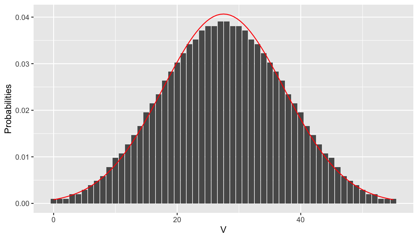
Figure 9.3: pmf of \(V\) when \(n = 10\) with superimposed normal distribution.

Example 9.1

Consider the normtemp data set in the fosdata package. Recall that this data is the gender, body temperature and heart rate of 130 patients. We are interested in whether the mean or median body temperature is 98.6. A \(t\)-test looks like this:

normtemp <- fosdata::normtemp
t.test(normtemp$temp, mu = 98.6)

## 
##  One Sample t-test
## 
## data:  normtemp$temp
## t = -5.4548, df = 129, p-value = 2.411e-07
## alternative hypothesis: true mean is not equal to 98.6
## 95 percent confidence interval:
##  98.12200 98.37646
## sample estimates:
## mean of x 
##  98.24923

resulting in a \(p\)-value of \(2 \times 10^{-7}\). If we instead perform the Wilcoxon signed rank test, we get

wilcox.test(normtemp$temp, mu = 98.6)

## 
##  Wilcoxon signed rank test with continuity correction
## 
## data:  normtemp$temp
## V = 1774.5, p-value = 1.174e-06
## alternative hypothesis: true location is not equal to 98.6

The \(p\)-value still leads to the same conclusion at most reasonable \(\alpha\) levels, but it is about 5 times as large as the \(t\)-test.

Both the one sample \(t\)-test and the Wilcoxon signed rank test are estimating the probability of obtaining data “this unlikely” or “more unlikely,” given that the null hypothesis is true. However, the two tests are summarizing what it means to be “this unlikely” in different ways. We will explore the pros and cons of the Wilcoxon signed rank test versus the one sample \(t\)-test in Sections 9.3 and 9.4.

9.2 Two sample Wilcoxon tests

In this section, we will explain how to use wilcox.test to compare two populations. We will split the discussion into the cases when the data is paired and when it is independent.

9.2.1 Paired two sample test

In many studies, observations are naturally paired. Each observation consists of two measurements coming from two different populations. For example, the two measurements might be test scores before and after studying, opinions of a married couple, or pairs of agricultural fields matched for similar soil and weather characteristics. Any setting from Section 8.6 where a paired \(t\)-test is appropriate may also be studied with a paired Wilcoxon test.

The paired two sample Wilcoxon test has the following hypotheses and assumptions:

• \(H_0\) : The two populations have the same distribution.
• \(H_a\) : The two populations have different distributions.

Assumptions 9.1 (for paired Wilcoxon test)

1. Subtracting measured values is possible and meaningful. We will need to assume that a difference of 2 is less than a difference of 3, for example.
2. The only dependence is between pairs of data points, one from each population. Unpaired observations are independent.

Under these assumptions, the differences in the paired values in the two populations will be a symmetric distribution under the null hypothesis. Therefore, assuming the null hypothesis is true, we can use the Wilcoxon signed rank test on the differences of the values between the two populations.

Example 9.2

The flint data set in the fosdata package gives the results of tap water lead testing during the Flint, Michigan water crisis in 2015.⁷⁰ In the study, households filled three sample collection bottles from their faucets. One bottle was filled at “first draw,” after the faucet had been off for 6 hours. The second and third bottles were filled after the faucet had been running for 45 seconds, and after it had been running for 2 minutes. All bottles were sent to a lab at Virginia Tech for lead testing.

Does the length of time that a faucet is left on influence the measurement of lead in the water coming from the faucets?

We restrict to two populations: the amount of lead in the water on first draw (Pb1) and the amount of lead in the water two minutes later (Pb3). This is paired data. It would be wrong to assume independence between these two measurements within one household in this experiment. A faucet that has high levels of lead at first draw is also likely to have higher levels of lead two minutes later.

A careful look at the data reveals two houses that have notes saying they were tested twice. It is unreasonable to expect those pairs of data points to be independent of each other, so we remove the observations that correspond to those houses. This is a reasonable thing to do, especially if the houses weren’t tested twice based on the outcome of the first test.

flint <- fosdata::flint
flint <- flint %>%
  filter(Notes == "")

The null hypothesis is that the distribution of Pb1 (lead draw in first sample) and Pb3 (lead draw after 2 minutes) are the same. Under the null hypothesis, the difference between values in Pb1 and Pb3 will be symmetric, so the assumptions of the Wilcoxon signed rank test are met on the differences.

We start by providing a histogram of the differences.

flint %>% ggplot(aes(x = Pb1 - Pb3)) +
  geom_histogram() +
  labs(title = "Difference in lead levels: first draw and after 2 minutes")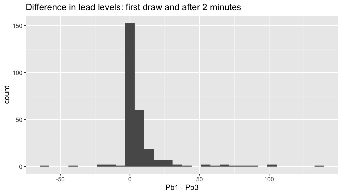

The histogram indicates that the difference in lead levels is positive and smallish, with a heavy right tail and outliers both positive and negative. The heavy tail and outliers make this data unsuitable for a \(t\)-test.

We perform the paired two sample Wilcoxon test as follows:

wilcox.test(flint$Pb1, flint$Pb3, paired = TRUE)

## 
##  Wilcoxon signed rank test with continuity correction
## 
## data:  flint$Pb1 and flint$Pb3
## V = 32931, p-value < 2.2e-16
## alternative hypothesis: true location shift is not equal to 0

The \(p\)-value is very low, so we reject \(H_0\) and conclude that running the water does make a significant difference to the lead level.

9.2.2 Independent two sample test

This section uses wilcox.test to compare independent samples from two populations, referred to as the Wilcoxon rank sum test. We no longer need to assume that the population distributions are symmetric, but we must assume that all of the observations are independent.

The null hypothesis and alternative hypotheses can be stated as follows.

• \(H_0\): the distribution of population one is the same as the distribution of population two.
• \(H_a\): the distribution of population one is different than the distribution of population two.

To perform the test, we choose a random sample of size \(m\) from population one and independently choose a random sample of size \(n\) from population two. For each data point \(x\) in group one, count the number of data points in group two that are less than \(x\). The total number of “wins” for group one (counting ties as 0.5) is the test statistic \(W\). Under the null hypothesis, the expected value of the test statistic is \[ E[W] = \frac{m n}{2}, \] which is exactly half of the possible pairings between the two groups.

Let’s look at a simple example for concreteness. Suppose that we obtain the following data, which has two observations in group one and three observations in group two.

group	value
1	5
1	11
2	0
2	3
2	10

The group one value \(x = 5\) is bigger than two observations in group two, and the group one value \(x = 11\) is larger than three observations in group two. So, the value of the test statistic is \(W = 2 + 3 = 5\). The expected value of the test statistic is \(2 \times 3 /2 = 3\). The \(p\)-value of the test is the probability (under the null) of obtaining a test statistic either 5 or larger, or obtaining one that is 1 or smaller, i.e., \(P(|W - 3| \ge 2)\). To compute this probability, we imagine that we have sorted the 5 values from smallest to largest. Under the null hypothesis, each possible arrangement of group one and group two within the sorted values would be equally likely. There are \(\binom{5}{3} = 10\) possible permutations of the values, shown as the ten rows of Table 9.2.

Table 9.2: Possible permutations of three 2’s and two 1’s, with associated test statistic.

V1	V2	V3	V4	V5	W
2	2	2	1	1	6
2	2	1	2	1	5
2	1	2	2	1	4
1	2	2	2	1	3
2	2	1	1	2	4
2	1	2	1	2	3
1	2	2	1	2	2
2	1	1	2	2	2
1	2	1	2	2	1
1	1	2	2	2	0

Under the assumption that the distribution of population one is the same as the distribution of population two, each outcome is equally likely. There are four rows of Table 9.2 with \(|W - 3| \ge 2\), so the \(p\)-value is \(P(|W - 3| \ge 2) = 4/10\).

The sampling distribution of the test statistic \(W\) is in R with root name wilcox, where as always, prefixes d, p, q, and r correspond to the pmf, cdf, quantile function, and random generator, respectively.

For example, if we wish to compute \(P(|W - 3| \ge 2)\) when the two sample sizes are 2 and 3 as above, we could do the following.

sum(dwilcox(c(0, 1, 5, 6), m = 2, n = 3))

## [1] 0.4

Figure 9.4 shows the distribution of the test statistic \(W\) with group sizes \(m = 5\) and \(n = 10\). The sampling distribution of the test statistic \(W\) is approximately normal when the groups are even modestly large.

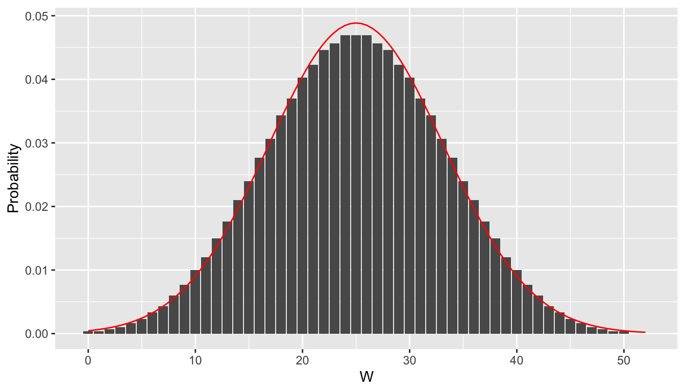
Figure 9.4: pmf of \(W\) when \(m = 5\), \(n = 10\), with superimposed normal distribution.

The function wilcox.test computes the test statistic \(W\) and the \(p\)-values in one simple step.

wilcox.test(c(5, 11), c(0, 3, 10))

## 
##  Wilcoxon rank sum exact test
## 
## data:  c(5, 11) and c(0, 3, 10)
## W = 5, p-value = 0.4
## alternative hypothesis: true location shift is not equal to 0

Example 9.3

Hillier et al.⁷¹ studied whether academic papers on climate change got more or fewer citations based on their narrative style. They assessed various aspects of the narrative style of the papers and also counted the number of citations. The data set climate in the fosdata package summarizes their data for articles published in three well-respected journals.

Let’s load the data and do some exploring.

climate <- fosdata::climate

For the purposes of this example, we are going to look at whether the distribution of articles with an appeal in the abstract are associated with different citation rates than those without an appeal. An appeal being “Yes” indicates that the author made an explicit appeal to the reader or a clear call for action. The normalized_citation variable gives the number of citations per year since publication. Let’s restrict to those two variables to clean things up a bit.

climate <- climate %>%
  select(binary_appeal, normalized_citations, abstract_number)

climate <- climate %>%
  mutate(climate,
    binary_appeal =
      factor(binary_appeal, levels = 0:1, labels = c("No", "Yes"))
  )
ggplot(climate, aes(x = binary_appeal, y = normalized_citations)) +
  geom_boxplot(outlier.size = -1) +
  geom_jitter(height = 0, width = 0.2)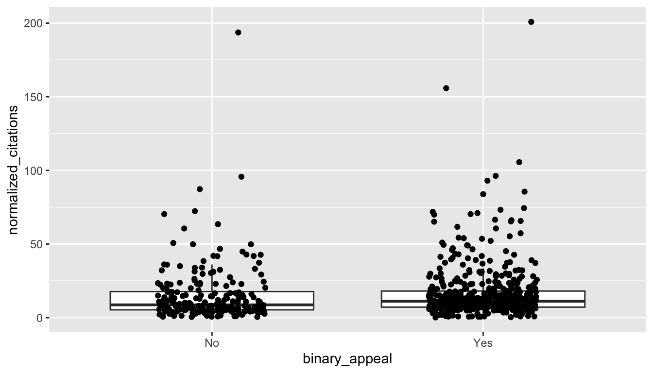

It’s a bit hard to see what is going on. Let’s compute some summary statistics.

climate %>%
  group_by(binary_appeal) %>%
  summarize(
    mean = mean(normalized_citations),
    sd = sd(normalized_citations),
    skew = e1071::skewness(normalized_citations),
    N = n()
  )

## # A tibble: 2 × 5
##   binary_appeal  mean    sd  skew     N
##   <fct>         <dbl> <dbl> <dbl> <int>
## 1 No             15.5  19.6  4.54   213
## 2 Yes            16.7  18.4  4.17   519

One thing that we notice is that there is quite a bit of skewness in these variables. The authors took the log of the citation variable, which lowered the skewness and made the data look more normal. A \(t\)-test without transforming the data would be problematic even with 200-500 samples because of the level of skewness of the data, as well as the outliers. Instead, we will use a Wilcoxon rank sum test with hypotheses:

• \(H_0\): the distribution of papers with an appeal is the same as the distribution of papers without an appeal.
• \(H_a\): the distribution of papers with an appeal is different than the distribution of papers without an appeal.

wilcox.test(normalized_citations ~ binary_appeal, data = climate)

## 
##  Wilcoxon rank sum test with continuity correction
## 
## data:  normalized_citations by binary_appeal
## W = 47608, p-value = 0.003182
## alternative hypothesis: true location shift is not equal to 0

Note the use of the formula notation ~ in wilcox.test; this is similar to its use in t.test, where we are telling R how we want to group the data. We reject the null hypothesis that the two distributions are the same at the \(\alpha = .05\) level.

Recall that the expected value of the test statistic is

213 * 519 / 2

## [1] 55273.5

The test statistic that we obtained is 47608, which is lower than the expected value. This indicates that the “no appeal” papers are cited less frequently than would be expected under the null hypothesis.

9.2.3 Ordinal data

Another common use of wilcox.test is when the data is ordinal rather than numeric.

Definition 9.4

Data is ordinal when, given data points \(p_1\) and \(p_2\), we can determine whether \(p_1\) is bigger than \(p_2\), less than \(p_2\), or equal to \(p_2\).

For example, airplane passengers may fly first class, business class, or coach. The seat type of an airline passenger is ordinal data because the three types of seats are ordered by quality.

Ordinal data is different from numeric data because there is no natural way to assign numbers to ordinal data. It is quite common to assign numbers to ordinal categories, but that doesn’t necessarily mean that it is a correct thing to do.

Example 9.5

Surveys commonly ask for responses in the form of Likert-scale data. The Likert scale is an ordinal five-point scale with choices reflecting agreement with a statement. Often, those options are given numeric values, as in this example:

Circle the response that most accurately reflects your opinion

Question	Strongly Agree	Agree	Neutral	Disagree	Strongly Disagree
Pride and Prejudice
is a great book	1	2	3	4	5
wilcox.test is a
useful R command	1	2	3	4	5

Although the options are listed as numbers, it does not necessarily make sense to treat the responses numerically. For example, if one respondent Strongly Disagrees that wilcox.test is useful, and another Strongly Agrees, is the mean of those responses Neutral? What is the mean of Strongly Agree and Agree? If the responses are numeric, what units do they have? So, it may not (and often does not) make sense to treat the responses to the survey as numeric data, even though it is encoded as numbers. For compelling examples of how numbering Likert scales can lead you astray, see the somewhat whimsical booklet, “Do not use averages with Likert scales.”⁷²

What we can do with Likert scale data is to order the responses in terms of amount of agreement. It is clear that Strongly Agree > Agree > Disagree > Strongly Disagree. Neutral is omitted because Neutral responses open a whole new can of worms. For example, we don’t know whether someone who put Neutral for Question (1) did so because they have never read Pride and Prejudice, or because they read it and don’t have an opinion on whether it is a great book. In one case, the response might better be treated as missing data, while in the other it would be natural to include the result between Agree and Disagree.

Example 9.6

Consider the MovieLens data set fosdata::movies from Chapter 6. Each movie review has a star rating, which is a subjective opinion of how much enjoyment the viewer had. The number of stars that a movie receives can definitely be ordered from 5 stars being the best, down to 1/2 star being the worst. It is not as clear that the number of stars should be treated numerically. To perform inference with the star ratings, we prefer the Wilcoxon test, which depends only on the ordinal nature of the data.

Let’s compare the movies Toy Story and Toy Story 2. Recall that the data that we have in our MovieLens data set is a random sample from all users. Is there sufficient evidence to suggest that there is a difference in the ratings of Toy Story and Toy Story 2 in the full data set?

The movies data set consists of observations pulled from 610 distinct users. If one user rates both Toy Story and Toy Story 2, those two ratings are not independent of each other. So, let’s recast the question as follows. Among those people who have only rated one or the other movie, is there evidence of a difference in the ratings of Toy Story and Toy Story 2 in the full data set?

We should also decide whether we want to do a one-sided or a two-sided test. Some people have strong opinions about which Toy Story movie is better, but that is not sufficient evidence or reason to do a one-sided test. So, let \(X\) be the rating of Toy Story for a randomly sampled person in the large data set who only rated one of the two movies. Let \(Y\) be the rating of Toy Story 2 for a randomly sampled person who only rated one of the two movies. Our null and alternative hypotheses are:

• \(H_0\): \(X\) and \(Y\) have the same distribution.
• \(H_a\): \(X\) and \(Y\) do not have the same distribution.

After loading the data, we create a data frame that only has the ratings of the first two Toy Story movies (by excluding Toy Story 3 which came out years later).

toy_story <- fosdata::movies %>%
  filter(stringr::str_detect(title, "Toy Story [^3]"))

Next, we filter out only those ratings from people who rated just one of the two movies.

toy_story_once <- toy_story %>%
  group_by(userId) %>%
  mutate(N = n()) %>%
  filter(N == 1)

Finally, we perform the Wilcoxon test:

wilcox.test(rating ~ title, data = toy_story_once)

## 
##  Wilcoxon rank sum test with continuity correction
## 
## data:  rating by title
## W = 1060.5, p-value = 0.9448
## alternative hypothesis: true location shift is not equal to 0

There is not a statistically significant difference (\(p = 0.94\)) between the ratings of Toy Story and Toy Story 2. We do not reject the null hypothesis.

9.3 Power and sample size

In this section, we compare the power of a \(t\)-test with that of a one sample Wilcoxon test. We do so with three populations: normal, heavy tails, and normal with an outlier.

We begin by comparing the power of Wilcoxon rank sum test with \(t\)-test when the underlying data is normal. We assume we are testing \(H_0: \mu = 1\) versus \(H_a: \mu \not= 1\) at the \(\alpha = .05\) level, when the underlying population is truly normal with mean 0 and standard deviation 1 with a sample size of 10. Let’s first estimate the percentage of time that a \(t\)-test correctly rejects the null-hypothesis.

mean(replicate(10000, t.test(rnorm(10, 0, 1), mu = 1)$p.value < .05))

## [1] 0.8011

We see that we correctly reject \(H_0\) 80.1% of the time in this simulation. Let’s see what happens with the Wilcoxon test.

mean(replicate(10000, wilcox.test(rnorm(10, 0, 1), mu = 1)$p.value < .05))

## [1] 0.7864

Here, we see that we correctly reject \(H_0\) 78.6% of the time in this simulation. If you repeat the simulations, you will see that indeed a \(t\)-test correctly rejects \(H_0\) more often than the Wilcoxon test does, on average.

However, if there is a departure from normality in the underlying data, Wilcoxon can outperform t.test. Let’s repeat the above simulations with a heavy tailed distribution. We sample from a \(t\) distribution with 3 degrees of freedom.

mean(replicate(10000, t.test(rt(10, 3), mu = 1)$p.value < .05))

## [1] 0.5378

mean(replicate(10000, wilcox.test(rt(10, 3), mu = 1)$p.value < .05))

## [1] 0.544

Here, we see that Wilcoxon outperforms \(t\), but not by a tremendous amount.

Finally, we look at the third example, which is normal with a single outlier. Our model for an outlier will be that we multiply one of the values by 100. This does not change the mean of the distribution (since it is still zero), but it will often introduce relatively large outliers. We can simulate data of this type as follows:

dat <- rnorm(10, 0, 1)
dat[10] <- dat[10] * 100
dat

##  [1]  -0.07719331   1.84950460  -0.08484561   0.09717147  -0.59400957
##  [6]  -0.60122548   0.55263885  -1.04205402  -0.09278696 -57.35763723

If you run the above code multiple times, you will see that the last value usually does not appear to come from a standard normal distribution, though sometimes it can appear to do so.

We again estimate the power of a \(t\)-test and a one sample Wilcoxon test on this type of data, again with \(H_0: \mu = 1\). Since the simulations are a bit more complicated, we write out the simulations in a longer format.

p_vals <- replicate(10000, {
  dat <- rnorm(10, 0, 1)
  dat[10] <- dat[10] * 100
  t.test(dat, mu = 1)$p.value
})
mean(p_vals < .05)

## [1] 0.033

p_vals <- replicate(10000, {
  dat <- rnorm(10, 0, 1)
  dat[10] <- dat[10] * 100
  wilcox.test(dat, mu = 1)$p.value
})
mean(p_vals < .05)

## [1] 0.4275

Now we see a substantial difference in the power of the two tests, with the one sample Wilcoxon test being much more powerful.

Alert 9.1

If your data is symmetric with outliers, the one sample Wilcoxon test will be much more powerful than the one sample \(t\)-test.

To summarize the results of this section:

1. If your population is normal, then a \(t\)-test will be a little bit more powerful than a one sample Wilcoxon test.
2. If your population has moderately heavy tails, then a one sample Wilcoxon test will likely be a little bit more powerful than a \(t\)-test.
3. If your population has outliers, you should use a one sample Wilcoxon test rather than a \(t\)-test.

9.3.1 Sample size

When performing rank-based tests, we recommend using simulation to estimate power and sample sizes. With power computations, we will set the significance level \(\alpha\) we wish to test, and we will need some estimate of the effect size we wish to detect. This can be challenging to do well. We illustrate the technique with an example.

Example 9.7

Suppose we are designing an experiment in which students are randomly assigned to either a traditional classroom or a flipped classroom. At the end of the semester, students will be given a statement and asked whether they Strongly Agree, Agree, Disagree or Strongly Disagree with the statement. We wish to determine whether there is a statistically significant difference in the responses between those in the traditional classroom and those in the flipped classroom. For an experiment with significance level \(\alpha = 0.05\) and power of 80%, what number of students would need to be assigned to each group?

To perform the simulation, we need to estimate the specific distribution of responses in the two groups under the alternate hypothesis. The power computation will tell us how large a sample we need to take to be able to detect the difference between our estimated distributions. Without knowledge of what sort of effect size matters to educational decisions, this is impossible. So imagine we read literature about educational studies, and decide that a reasonable effect would be probability distributions given in the table below.

	Traditional	Flipped
Strongly Agree	0.4	0.6
Agree	0.3	0.3
Disagree	0.1	0.1
Strongly Disagree	0.2	0.0

We recommend estimating the power for various sample sizes and plotting a smoothed version of the resulting curve. When using this technique, we don’t need to estimate each probability as accurately as we would if we were only doing it once.

p_trad <- c(.4, .3, .1, .2)
p_flip <- c(.6, .3, .1, 0)

sample_sizes <- seq(10, 150, length.out = 20)
powers <- sapply(sample_sizes, function(x) {
  tt <- replicate(500, {
    d1 <- sample(1:4, x, T, prob = p_trad)
    d2 <- sample(1:4, x, T, prob = p_flip)
    suppressWarnings(wilcox.test(d1, d2))$p.value
  })
  mean(tt < .05)
})
for_plot <- data.frame(
  sample_size = sample_sizes,
  power = powers
)

ggplot(for_plot, aes(x = sample_size, y = power)) +
  geom_smooth(se = F) +
  geom_point()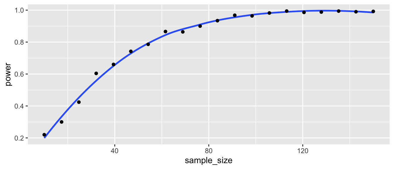

We read off of the plot that in order to have a power of about 0.8, we would need about 58 samples in each group.

9.4 Effect size and consistency

9.4.1 Effect size

When communicating statistical results to others, it may be useful to include a common language effect size. The goal of a common language effect size statistic is to present results in a way that is easy to understand without advanced statistical training. We recommend the following for the two sample Wilcoxon rank sum test.

Definition 9.8

Given two populations, Vargha and Delaney’s \(A\) is the probability that a sample from one population will be larger than a sample from the other population plus one-half the probability that they will be equal.

Intuitively, Vargha and Delaney’s \(A\) is the probability that a sample from one population will be larger than a sample from the other population, where we are assuming that ties are broken 50-50.

The effect size \(A\) is directly related to the test statistic for the two sample Wilcoxon rank sum test. The Wilcoxon test statistic \(W\) counts the number of times that samples from population one are larger than those in population two, plus one half the number of ties. To compute \(A\), divide \(W\) by the number of comparisons that are made.

Example 9.9

Let’s make sense of the difference between Sense and Sensibility (1995) and The Sixth Sense (1999), the two most popular movies with “sense” in the title. The corresponding movieId’s for those movies are 17 and 2762. Which movie is preferred, is there a significant difference, and what is the effect size?

To maintain independence of the samples, restrict to those raters who only rated one of the two movies:

sensible_movies <- fosdata::movies %>%
  filter(movieId %in% c(17, 2762)) %>%
  group_by(userId) %>%
  mutate(N = n()) %>%
  filter(N == 1)

Now test whether the distribution of ratings are the same for these two sensible movies:

wilcox.test(rating ~ title, data = sensible_movies)

## 
##  Wilcoxon rank sum test with continuity correction
## 
## data:  rating by title
## W = 3089.5, p-value = 0.65
## alternative hypothesis: true location shift is not equal to 0

The \(p\)-value is 0.65, so there is not a significant difference in the ratings. For the common language effect size \(A\), we need to know the number of comparisons. How many ratings of each sensible movie were there?

table(sensible_movies$title)

## 
## Sense and Sensibility (1995)      Sixth Sense, The (1999) 
##                           42                          154

Since each pair of ratings is compared, there are \(42 \times 154 = 6468\) comparisons. Then \(A = W / 6468 = 3089.5 / 6468 \approx 47.8\%\). Since Sense and Sensibility comes first in the ordering of titles, Sense and Sensibility is preferred by about 47.8% of raters, while The Sixth Sense is preferred by about 53.2% of raters. (This is only formally true if we imagine that for ties we flip a coin.)

Without using the \(W\) statistic, we can compute \(A\) directly:

s_and_s_ratings <- filter(sensible_movies, movieId == 17) %>%
  pull(rating)
t_s_s_ratings <- filter(sensible_movies, movieId == 2762) %>%
  pull(rating)
sum(sapply(s_and_s_ratings, function(x) {
  sum(x > t_s_s_ratings) + 1 / 2 * sum(x == t_s_s_ratings)
})) / (length(s_and_s_ratings) * length(t_s_s_ratings))

## [1] 0.4776592

There is a package, effsize, that has a function to compute Vargha and Delaney’s \(A\) from the data with no manipulation:

effsize::VD.A(rating ~ title, data = sensible_movies)

## 
## Vargha and Delaney A
## 
## A estimate: 0.4776592 (negligible)

It’s still 47.8% in favor of Sense and Sensibility, described as a “negligible” effect. You should take the adjectives assigned to effect sizes by the effsize package with a grain of salt, as effect sizes are domain dependent. As with Cohen’s \(d\), what is considered a negligible effect in one field might be considered a large effect in a different field.

9.4.2 Consistency

In this section, we discuss the consistency of the one sample t.test and the two independent sample wilcox.test.

Definition 9.10

A hypothesis test is consistent if the probability of rejecting the null hypothesis given that the null hypothesis is false converges to 1 as the sample size goes to infinity.

Consistency is a desirable property for a hypothesis test because it means that a sufficiently large sample size will always have the power to detect a false \(H_0\). We will not provide proofs of consistency, but instead examine it via simulations.

Example 9.11

Consider the t.test with one population, where we are testing \(H_0: \mu = 0\) versus \(H_a: \mu \not= 0\). We assume that the underlying population has mean \(\mu_a \not= 0\), so \(H_0\) is false. Also assume the population is normally distributed with standard deviation \(\sigma = 1\), and choose significance level \(\alpha = 0.01\).

We start by computing the percentage of times \(H_0\) will be rejected when \(\mu_a = 1\) and the sample size is \(n = 20\).

sigma <- 1
nsize <- 20
mua <- 1
pvals <- replicate(10000, {
  dat <- rnorm(nsize, mua, sigma)
  t.test(dat, mu = 0)$p.value
})
mean(pvals < .01)

## [1] 0.9338

We see that with 20 samples, we already reject \(H_0\) about 93% of the time. By repeating this simulation with various values of \(n\) and \(\mu_a\), we create the plot in Figure 9.5. It appears that the probability of rejecting \(H_0\) is getting larger as the sample size increases, and it also appears to be converging to 1. We would need to take more samples to see this for \(\mu_a = 0.02\), but 0.02 is a very small difference between the null and alternative hypothesis.

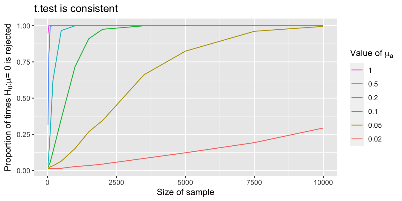
Figure 9.5: Each curve shows the probability that a \(t\)-test rejects \(H_0\) as sample size grows. The different curves correspond to different population means \(\mu_a\). As \(\mu_a\) gets closer to the hypothesized \(\mu = 0\), larger samples are needed to detect the difference.

The story for the Wilcoxon rank sum test is a bit more involved. We begin with an example where the null hypothesis is false, but we see that the test is not consistent.

Example 9.12

Let population 1 consist of numbers uniformly distributed on \([-1, 1]\). Let population 2 consist of numbers uniformly distributed on \([-2, -1]\) with probability \(1/2\), and numbers uniformly distributed on \([1,2]\) with probability \(1/2\), as shown.

Fixing \(\alpha = 0.05\), let’s see what percentage of times, on average, the Wilcoxon test rejects \(H_0\) with a sample size of \(n = 100\).

N <- 100
sim_data <- replicate(10000, {
  d1 <- runif(N, -1, 1)
  d2 <- sample(c(-1, 1), N, replace = TRUE) * runif(N, 1, 2)
  wilcox.test(d1, d2)$p.value
})
mean(sim_data < .05)

## [1] 0.0889

We see that the test rejects \(H_0\) more than with probability \(\alpha = .05\), but the test still has very low power. In other words, it does not do a good job of distinguishing population 1 from population 2. Repeating the computation with different sample sizes \(n\) produces Table 9.3.

Table 9.3: Power of Wilcoxon test.

n	power
10	0.105
20	0.098
50	0.125
100	0.092
200	0.107
500	0.101
1000	0.106

From Table 9.3 we see that as \(n\) grows, the power of the test is not approaching 1. It can be shown that when \(n \to \infty\), the power converges to about \(0.1095\). With these populations, the Wilcoxon rank sum test is not consistent.

However, we do have the following theorem:

Theorem 9.1

Suppose \(X\) and \(Y\) are random variables with finite variance and \[ P(X > Y) \not= P(X < Y). \] Then the Wilcoxon rank sum test of \(X\) against \(Y\) is consistent. That is, as the number of samples goes to infinity, the power converges to 1.

The condition in Theorem 9.1 is equivalent to a statement about Vargha and Delaney’s \(A\). If \(A \neq 0.5\), then the two sample Wilcoxon test is consistent.

Alert 9.2

We recommend using the Wilcoxon rank sum test only when we suspect, or wish to detect, a difference in populations that is of the type \(P(X > Y) \not= P(X < Y)\). In this case, the test is consistent.

To finish off this section, we provide an example of two populations such that \(P(X > Y) \not= P(X < Y)\), and give evidence with simulation that the Wilcoxon rank sum test is consistent.

Example 9.13

Let \(X\) and \(Y\) be random variables, with \(X \sim \text{Unif}(1,2)\) and \(Y\) taking values 0 and 3 with probabilities \(p < 1/2\) and \(1-p\). Then \(P(X > Y) = p\) and \(P(X < Y) = 1-p\). Fix significance level \(\alpha = 0.01\).

Here is a single computation when \(p = 0.4\) and the sample size \(n = 100\).

p <- 0.4
N <- 100
pvals <- replicate(1000, {
  x <- runif(N, 1, 2)
  y <- sample(c(0, 3), size = N, prob = c(p, 1 - p), replace = TRUE)
  suppressWarnings(wilcox.test(x, y))$p.value
})
mean(pvals < 0.01)

## [1] 0.416

The probability of correctly rejecting \(H_0\) in this case is 0.416. Repeating the simulation for different values of \(p\) and \(n\) produces the plot shown in Figure 9.6. From the figure, it appears that the percentage of times \(H_0\) is rejected converges to 1 as the sample size goes to infinity, so the test is consistent. Values of \(A\) closer to \(1/2\) require larger sample sizes.

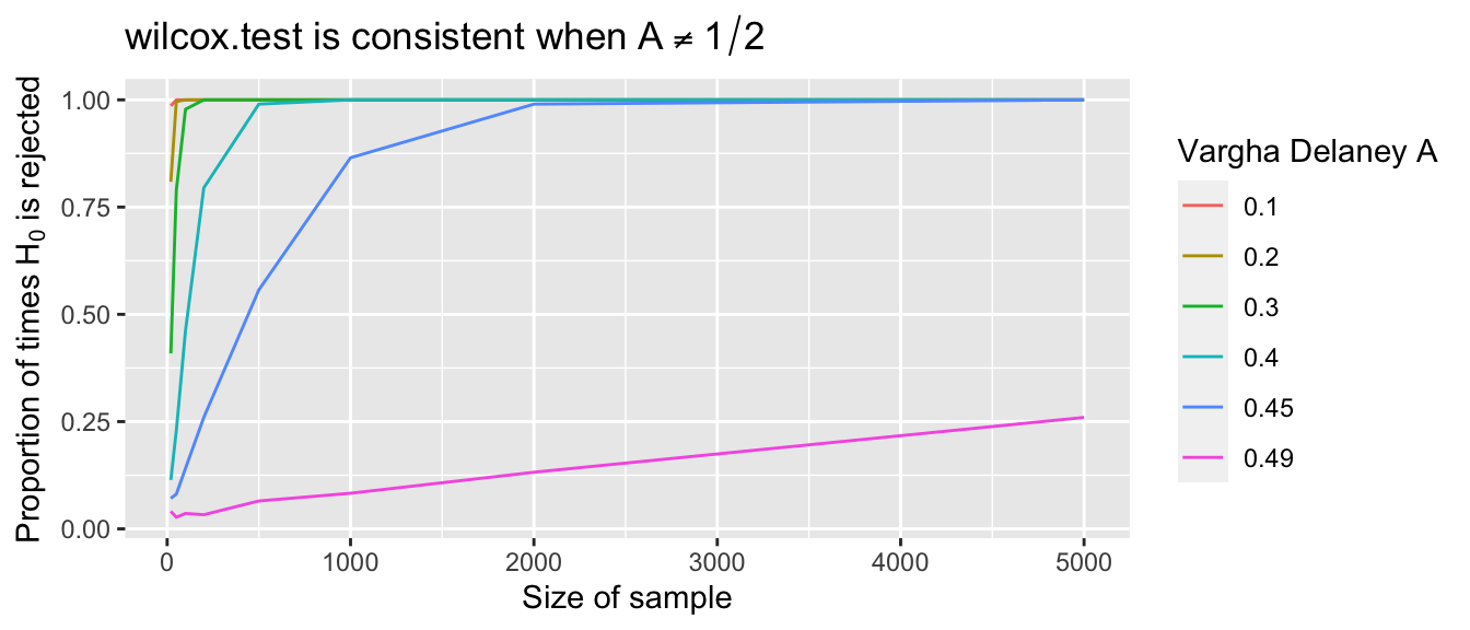
Figure 9.6: Each curve shows the probability that a Wilcoxon test rejects \(H_0\) as sample size grows. The curves correspond to fixed population values of \(A = P(X < Y)\). As \(A\) gets closer to 1/2, larger samples are needed to detect the difference between \(X\) and \(Y\).

9.5 Summary

In this chapter, we provided an alternative to t.test. In the one sample case, we can use the Wilcoxon signed rank test for a random sample from a symmetric population. The Wilcoxon signed rank test is preferred over t.test when either the data is ordinal and means cannot be taken, or when in the presence of outliers. For a population that is normally distributed, use t.test because it has slightly larger power. When the population distribution is skewed or unknown (but with no outliers), use t.test with the caveats regarding sample size presented in Chapter 8.

In the independent two sample case, we can use the Wilcoxon rank sum test as an alternative to t.test. Use the Wilcoxon rank sum test when the data is ordinal, when there may be outliers, or when the sample sizes are small enough that the Central Limit Theorem may not apply. Recall that the sample size required for the Central Limit Theorem to apply depends on the distribution. Use t.test when the populations are normal or when the sample size is large enough that the Central Limit Theorem applies. If the data is ordinal, but can be transferred meaningfully to a numeric scale, then you can use t.test on the transferred data. However, it can be difficult to re-interpret your result in the original scale when you do this.

For the two sample Wilcoxon rank sum test, the null hypothesis is that the populations are the same and the alternative is that they are different. The power of a Wilcoxon rank sum test goes to 1 as the sample size goes to infinity in the case that \(P(X > Y) \not= P(X < Y)\). We recommend only using the Wilcoxon rank sum test when you wish to detect differences between the populations of the type \(P(X > Y) \not= P(X < Y)\). If the null hypothesis is rejected, then we recommend reporting Vargha and Delaney’s \(A\) as an estimate of effect size, and as an estimate of \(P(X > Y)\). If the populations appear to be different for reasons other than \(P(X > Y) \not= P(X < Y)\), such as having different variances, then the Wilcoxon rank sum test will typically have poor power, and should not be used. For a more advanced theoretical treatment of this topic, we recommend the text by Lehmann.⁷³

In the paired two sample case, we can use the Wilcoxon signed rank test on the differences as an alternative to a \(t\)-test on the differences. For the Wilcoxon signed rank test to be valid, the differences in values must be meaningful, and in particular, must satisfy the conditions of the Wilcoxon signed rank test. Use Wilcoxon signed rank when the data is ordinal with meaningful differences or when there are outliers.

Vignette: ROC curves and the Wilcoxon rank sum statistic

Suppose you wish to classify an object into one of two groups. It would be helpful if there were a variable \(X\) and a value \(x_0\) such that whenever \(X < x_0\) we would classify the object into group 1, and whenever \(X \ge x_0\) we would classify the object into group 2. A receiver operating characteristic (ROC) curve is a graphical measurement of how well a variable discriminates between two alternatives.

As an example, let’s consider palmerpenguins::penguins and suppose that we are trying to distinguish between Adelie and chinstrap penguins, based solely on bill length.

penguins <- palmerpenguins::penguins %>%
  filter(species %in% c("Adelie", "Chinstrap")) %>%
  mutate(species = droplevels(species))
ggplot(
  penguins,
  aes(x = bill_length_mm, y = flipper_length_mm, color = species)
) +
  geom_point() +
  geom_vline(xintercept = c(40.9, 46), linetype = "dashed")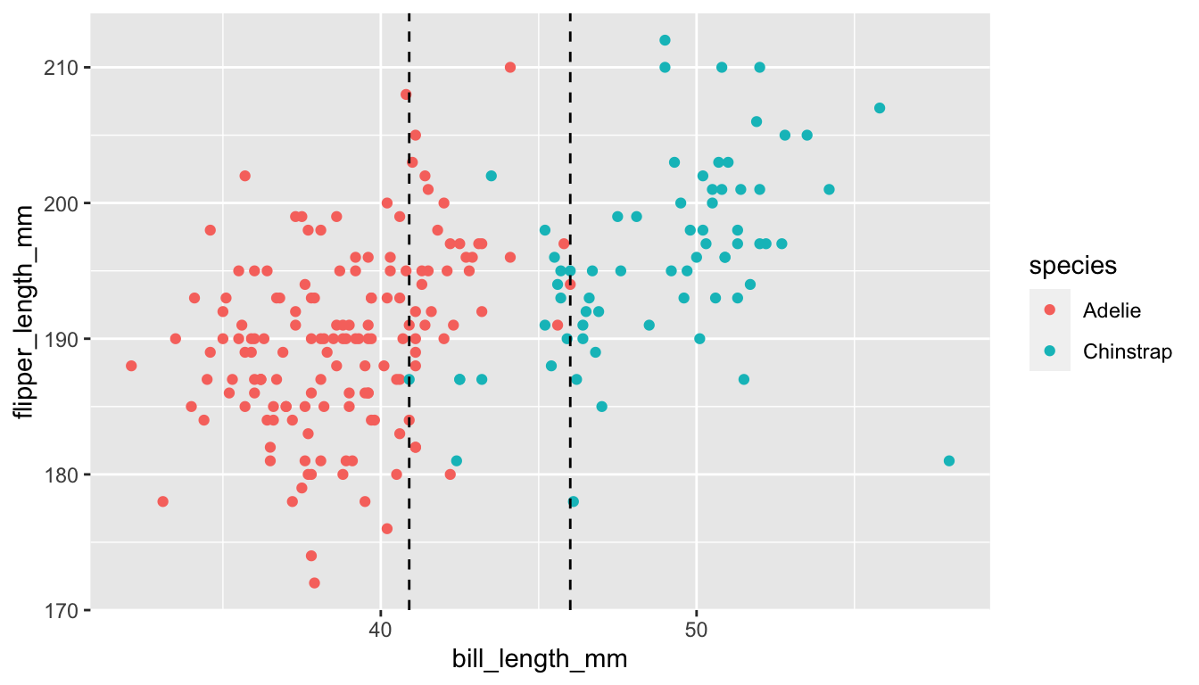

Based on this graph, we can see that there is not a value of bill length that completely separates the two variables. Whatever \(x_0\) we pick so that we assign any penguin with bill length less than \(x_0\) to be Adelie, we will be misclassifying some of the penguins. The ROC curve is computed as follows. Start at the smallest bill length and imagine that is your split value; all penguins with bill length less than that are classified as Adelie. The \(y\)-coordinate is the percentage of penguins correctly classified as Adelie with that split value, and the \(x\)-coordinate is the percentage of penguins incorrectly classified as Adelie with that split value.

An ideal ROC curve would look like this:

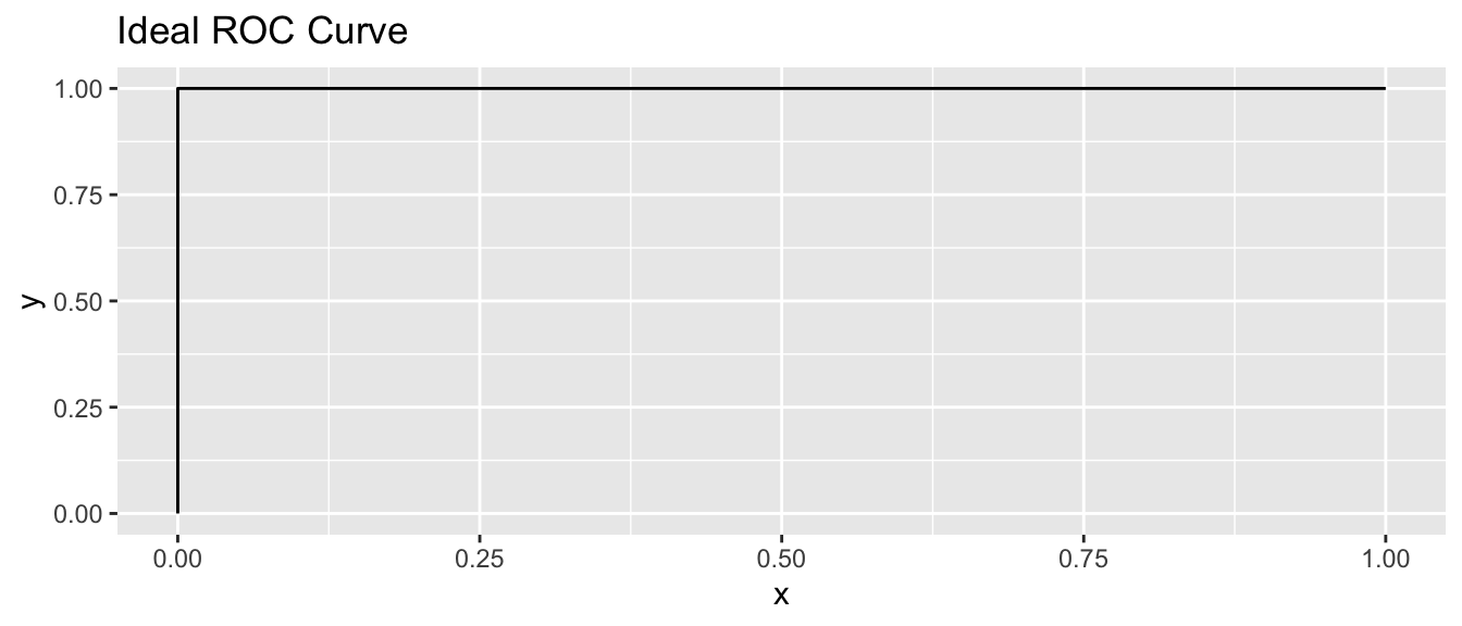
This means that there is at least one \(x_0\) such that all of the objects in group 1 have values less than \(x_0\), while all of the objects in group 2 have values at least \(x_0\). Let’s look at the ROC curve for the penguins using the ROCR package.

penguins <- penguins %>% select(species, bill_length_mm)
penguins <- penguins[complete.cases(penguins), ]
pred <- ROCR::prediction(penguins$bill_length_mm, penguins$species)
perf <- ROCR::performance(pred, "tpr", "fpr")
plot(perf, colorize = TRUE, main = "ROC curve for two penguin species")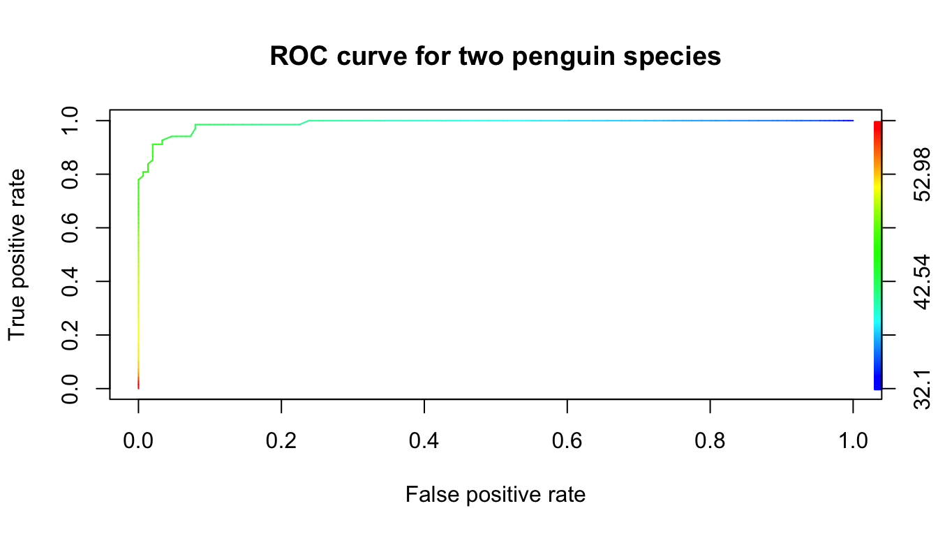

Note that the curve looks similar to the idealized version, except that it cuts off the corner at the top left. The curve there is green, which corresponds to bill lengths of around 45 mm. Those values of bills are exactly where we are unsure how the penguin should be classified.

The area underneath an ideal ROC curve is 1. For the penguin ROC curve, a little bit of area is missing in the upper left corner. The area under the ROC curve is abbreviated AUC and measures the separation between the two groups. It is used as a performance measure for machine learning algorithms.

Proposition 9.1

The area under the ROC curve (AUC) is equal to Vargha and Delaney’s \(A\).

Proposition 9.1 allows another interpretation of the AUC: it measures the probability that a randomly selected member of group 2 has a higher value of the variable under question than a randomly selected member of group 1. We will not prove Proposition 9.1, but the following code verifies that three ways of computing the AUC are the same in this context.

penguins <- penguins %>%
  mutate(species = factor(species, levels = c("Chinstrap", "Adelie")))
wilcox.test(bill_length_mm ~ species, data = penguins)$statistic / (151 * 68)

##         W 
## 0.9901636

effsize::VD.A(bill_length_mm ~ species, data = penguins)

## 
## Vargha and Delaney A
## 
## A estimate: 0.9901636 (large)

perf <- ROCR::performance(pred, "auc")
perf@y.values[[1]]

## [1] 0.9901636

Exercises

Exercises 9.1 – 9.6 require material through Section 9.1.

9.1

Suppose you wish to test \(H_0: \mu = 2\) versus \(H_a: \mu \not= 2\) using a Wilcoxon signed rank test. If you collect 30 samples, what is the expected value of the test statistic \(V\) under the null hypothesis?

9.2

Suppose you are testing \(H_0: \mu = 0\) versus \(H_a: \mu \not= 0\). You collect 40 data points and compute \(V = 601\). Use the built-in R function dsignrank or psignrank to compute the \(p\)-value associated with the test.

9.3

Suppose \(x_1,\ldots,x_n\) is a random sample from a symmetric distribution with mean 0.

1. Show that the expected value of the Wilcoxon test statistic \(V\) is \(\displaystyle E(V) = \frac{n(n+1)}{4}\).
2. Find \(\displaystyle \lim_{x_n\to \infty} E[V]\), which is the scenario of a single, arbitrarily large outlier.

9.4

Suppose you wish to test \(H_0:\mu = 3\) versus \(H_a: \mu\not= 3\). You collect the data points \(x_1 = -4\), \(x_2 = 0\), \(x_3 = 2\) and \(x_4 = 8\). Go through all of the steps of a Wilcoxon signed rank test and determine a \(p\)-value. Check your answer using R.

9.5

In this example, we explore what happens when applying the Wilcoxon signed rank test to skewed data. Suppose you take a random sample of size 20 from an exponential random variable with rate 1. The mean of the distribution is 1, and the median is \(\log(2)\). All tests below are to be conducted at the \(\alpha = .05\) level.

1. Estimate the effective type I error when testing \(H_0: \mu = 1\) versus \(H_a: \mu \not= 1\) in this setting.
2. Estimate the effective type I error when testing \(H_0: m = \log(2)\) versus \(H_a: m \not= \log(2)\) in this setting.
3. Even though the test is not working correctly for either of those values, there is a value that makes the test work approximately correctly. The value is called a pseudo-median, and for exponential random variables with rate 1 it is approximately 0.84. Confirm that the effective type I error of testing \(H_0: m = .84\) versus \(H_a: m \not= .84\) is approximately 0.05. (It is, based on our simulations, slightly larger than .05.)

9.6

Consider the weight_estimate data set in the fosdata package. Children, and some adults, were asked to estimate the weight of an object while watching a professional actor pick it up. For the purposes of this problem, consider only the mean200 variable.

1. Plot a boxplot of mean200. Does it appear to be reasonable symmetric?
2. Conduct a Wilcoxon signed rank test of \(H_0: \mu = 200\) versus \(H_a: \mu \not= 200\) at the \(\alpha = .05\) level and interpret.

---

Exercises 9.7 – 9.16 require material through Section 9.2.

9.7

Suppose you wish to perform a two sample Wilcoxon rank sum test. You collect data \(x_1 = 2, x_2 = 6\) and \(y_1 = 4, y_2 = 9\) and \(y_3 = 10\). Compute the test statistic and \(p\)-value by hand, and check your answer using R.

9.8

On episode 2 of the Nicolas Cage documentary, “The History of Swear Words,” six comedians took part in an experiment. Each was asked to submerge their hand in a bucket of ice water for as long as they could stand it. Four of the comedians were allowed to swear out loud while performing the experiment, the other two were forbidden from swearing. The two clean subjects spent 53 and 58 seconds in the water, while the four swearing comedians spent 69, 78, 87, and 140 seconds in the water.

1. Test for a difference between the two groups using a Wilcoxon rank sum test and report your \(p\)-value.
2. Repeat your analysis with a \(t\)-test.
3. What happens if you change to a one-sided hypothesis?
4. Were any of your analyses significant at the \(\alpha = 0.05\) level? What conclusions would you draw from this experiment?

9.9

The data set fosdata::bechdel is described in Example 7.4.

1. Make a boxplot comparing the distributions of budget_2013 for movies that pass and movies that fail the binary Bechdel test.
2. Perform a Wilcoxon rank sum test to compare the budgets of movies that pass the Bechdel test with movies that fail. Report your conclusion with a \(p\)-value.
3. Explain why a \(t\)-test would be inappropriate to use with this data.

9.10

In 1876, Charles Darwin studied the growth of pairs of corn seedlings, one produced by cross-fertilization and the other produced by self-fertilization. These seedlings were grown in pairs, with one of each type planted under the same conditions in the same pot. The final heights of the plants are in the cross and self variables of the data ZeaMays in the HistData package.

1. Make a boxplot to compare the distribution of heights of cross- and self-fertilized plants.
2. Why would a rank based test be preferable to a \(t\)-test for this data?
3. Carry out an appropriate rank based test to compare the two groups and state your conclusion with a \(p\)-value.

9.11

In an experiment, 37 volunteers with influenza or influenza symptoms were observed, each with and without a face mask. Experimenters measured the number of fine influenza particles in both settings. The data is available in fosdata::masks.

1. Make a plot or plots to confirm that the mask_fine and no_mask_fine variables are highly skewed and inappropriate for a \(t\)-test.
2. Does a \(t\)-test detect a difference in particles for the mask and no mask conditions?
3. Does a Wilcoxon test detect a difference in particles for the mask and no mask conditions?
4. Transform both variables by \(x \to \log(1 + x)\) and check that they would now be reasonable to use in a \(t\)-test.
5. Does a \(t\)-test detect a difference in particles for the mask and no mask conditions, after the \(\log(1+x)\) transformation?
6. Overall, does it appear that wearing a mask reduces the number of fine influenza particles?

9.12

This exercise explores how the Wilcoxon test changes when data values are transformed.

1. Suppose you wish to test \(H_0: \mu = 0\) versus \(H_a: \mu \not = 0\) using a Wilcoxon test You collect data \(x_1 = -1,x_2 = 2,x_3 = -3,x_4 = -4\) and \(x_5 = 5\). What is the \(p\)-value?
2. Now, suppose you multiply everything by 2: \(H_0: \mu = 0\) versus \(H_a: \mu\not = 0\) and your data is \(x_1 = -2,x_2 = 4,x_3 = -6,x_4 = -8\) and \(x_5 = 10\). What happens to the \(p\)-value? (Try to answer this without using R. Check your answer using R, if you must.)
3. Now, suppose you square the magnitudes of everything. \(H_0: \mu = 0\) versus \(H_a: \mu \not= 0\), and your data is \(x_1 = -1,x_2 = 4,x_3 = -9,x_4 = -16\) and \(x_5 = 25\). What happens to the \(p\)-value?
4. Compare your answers to those that you got when you did the same exercise for \(t\)-tests in Exercise 7.8.

9.13

Consider the data in ex0221 in the Sleuth3 package. This data gives the humerus length of 24 adult male sparrows that perished in a winter storm, as well as the humerus length of 35 adult male sparrows that survived. The question under consideration is whether those that perished did so because of some physical characteristic; measured in this case by humerus length.

1. Create a boxplot of humerus length for the sparrows that survived and those that perished. Note that there is one rather extreme outlier in the Perished group.
2. Use a Wilcoxon rank sum test to test whether the median humerus length is the same in both groups.
3. Is there evidence to conclude that the humerus length is different in the two groups?

9.14

Consider the data in ex0428 in the Sleuth3 package. This gives the plant heights in inches of plants of the same age, one of which was grown from a seed from a cross-fertilized flower, and the other of which was grown from a seed from a self-fertilized flower.

1. Is there a significant difference in the height of the flowers at the \(\alpha = .05\) level?
2. Create a boxplot of the height of the flowers for each type of fertilization. Comment on any abnormalities apparent. (Hint: this data is in “wide” format rather than “long” format, and you may want to use pivot_longer to convert it.)

9.15

The data set malaria from the ISwR package contains 100 observations of children in Ghana. (Note: this is not the same as the malaria data set from the fosdata package!) The data records each child’s age, levels of a particular antibody, and whether or not they have malaria symptoms.

1. State and carry out a hypothesis test that the antibody levels (ab) differ between the groups with and without malaria symptoms. Use the Wilcoxon rank sum test.

2. Inspect a boxplot or histogram of the ab variable by mal. Would you use this variable in a \(t\)-test? Explain.

3. Inspect a boxplot or histogram of \(\log(\text{ab})\) by mal. Would you use this variable in a \(t\)-test? Explain.

4. Carry out a \(t\)-test that the log of antibody levels differ between malaria groups and compare your results to the Wilcoxon test.

9.16

The data set flint from the fosdata package contains data on lead in tap water from Flint, Michigan in 2015. Is there a difference in the mean lead level after running water for 45 seconds (Pb2) and for 2 minutes (Pb3)?

1. Explain why it is very likely that each observation of Pb2 is dependent on the observation of Pb3.
2. There are two houses that are sampled twice. What does this imply about the independence of Pb2 and Pb3 between observations? Since this only affects 4 of the 271 observations, we will ignore this.
3. Plot the data. Would it be appropriate to use a \(t\)-test directly on this data?
4. If appropriate, test using a Wilcoxon signed rank test at the \(\alpha = .01\) level.
5. State your conclusions, including either a point estimate or a confidence interval for the pseudo-median (see Exercise 9.5 on the difference in lead levels).

---

Exercises 9.17 – 9.21 require material through Section 9.3.

9.17

Compare the effective power of t.test versus wilcox.test in the case of testing \(H_0: \mu = 0\) versus \(H_a: \mu \not= 0\) when the underlying population is uniform on the interval \([-0.5, 1]\), and the sample size is 30.

9.18

This problem explores the effective type I error rate for a one sample Wilcoxon and \(t\)-tests. Choose a sample of 21 values where \(X_1,\ldots,X_{20}\) are iid normal with mean 0 and sd 1, and \(X_{21}\) is 10 or -10 with equal probability. Test \(H_0: m = 0\) versus \(H_a: m\not= 0\) at the \(\alpha = .05\) level. How often does the Wilcoxon test reject \(H_0\)? Compare with the effective type I error rate for a \(t\)-test of the same data. Which test is performing closer to how it was designed?

9.19

How well can hypothesis tests detect a small change? Suppose the population is normal with mean \(\mu = 0.1\) and standard deviation \(\sigma = 1\). We test the hypothesis \(H_0: \mu = 0\) versus \(H_a: \mu \neq 0\).

1. When \(n = 100\), what percent of the time does a \(t\)-test correctly reject \(H_0\)?
2. When \(n = 100\), what percent of the time does a Wilcoxon test correctly reject \(H_0\)?
3. Repeat parts (a) and (b) with \(n = 1000\).
4. The assumptions for both tests are satisfied, since the population is normal. Which test would you recommend?

9.20

In this problem, we estimate the probability of a type II error. Suppose you wish to test \(H_0:\mu = 1\) versus \(H_a: \mu\not=1\) at the \(\alpha = .05\) level.

1. Suppose the true underlying population is \(t\) with 3 degrees of freedom, and you take a sample of size 20.
   1. What is the true mean of the underlying population?
   2. What type of error would be possible to make in this context, type I or type II? In the problems below, if the error is impossible to make in this context, the probability would be zero.
2. Approximate the probability of a type I error if you use a \(t\)-test.
3. Approximate the probability of a type I error if you use a Wilcoxon test.
4. Approximate the probability of a type II error if you use a \(t\)-test.
5. Approximate the probability of a type II error if you use a Wilcoxon test.
6. Note that \(t\) random variables with small degrees of freedom have heavy tails and contain data points that look like outliers. Does it appear that Wilcoxon or \(t\)-test is more powerful with this type of population?

9.21

Suppose that you are planning an experiment, and you wish to use a two sample Wilcoxon test on your data. You wish your experiment to have power of 80% when the test is performed at the \(\alpha = .05\) level and when population one is normal with mean 0 and standard deviation 1, and population 2 is normal with mean 0.4 and standard deviation 1. Assume that you will take equal sample sizes from each population.

Create a power versus sample size plot for 5 to 10 sample sizes between 20 and 200, and indicate how many samples from each population you would recommend.

---

Exercises 9.22 – 9.27 require material through Section 9.4.

9.22

Consider the MovieLens data fosdata::movies.

1. Is there sufficient evidence at the \(\alpha = .05\) level to conclude that among people who have only seen one of the movies, those people have a preference between Sleepless in Seattle and While You Were Sleeping?
2. Report Vargha and Delaney’s \(A\) effect size for this data, and interpret.

9.23

Consider the sharks data in the fosdata package.⁷⁴ Participants either watched a video or listened to an audio documentary about sharks while different types of music played. Participants were then asked to rate sharks on various dimensions such as gracefulness and viciousness. For this problem, consider only those participants who watched a video and heard either ominous or uplifting music.

1. Is there a difference in those participants’ responses to how vicious sharks are? Test at the \(\alpha = .05\) level.
2. If there is a difference, provide the common language effect size and explain.

9.24

Consider the plastics data set in the fosdata package. Snow was filtered in both the Arctic and Europe to find microfibers, which are microplastics that are in fibrous shape.

1. Perform a two sample Wilcoxon rank sum test to determine whether the length of the microfibers is the same in the Arctic as in Europe.
2. The authors in the paper⁷⁵ reported a test statistic of 13723, which is not what R reports. Confirm that the authors used the following method to obtain their test statistic. They computed the test statistic \(W\) from wilcox.test and then added the total number of comparisons between lengths of fibers from the Arctic with other lengths of fibers from the Arctic.
3. Provide an effect size in terms of Vargha and Delaney’s \(A\) and interpret.

9.25

Provide an estimate for the effect size in Exercise 9.16 and interpret.

9.26

Use simulation to show that if population 1 is standard normal, and population 2 is normal with mean 1 and standard deviation 1, then the Wilcoxon rank sum test is consistent at the \(\alpha = .05\) level.

9.27

Suppose population 1 is standard normal, and population 2 is normal with mean 0 and standard deviation 5.

1. Use simulation to show that \(P(X > Y) = .5\), where \(X\) is a random sample from population 1 and \(Y\) is a random sample from population 2.
2. Use sample sizes of \(n = 10, 100, 1000\) and 5000 for each population, and estimate the probability that the null hypothesis will be rejected at the \(\alpha = .05\) level. Use 1000 replications rather than 10,000 so that it runs in a reasonable amount of time.
3. Does the Wilcoxon rank sum test appear to be consistent in this context?

---

68. Donald K Milton et al., “Influenza Virus Aerosols in Human Exhaled Breath: Particle Size, Culturability, and Effect of Surgical Masks,” PLOS Pathogens 9, no. 3 (March 2013): 1–7, https://doi.org/10.1371/journal.ppat.1003205.↩︎

69. A dotplot is similar to a histogram, with each data point shown as an individual dot. This one was made with geom_dotplot.↩︎

70. Rebekah Martin et al., “Lead Results from Tap Water Sampling in Flint, MI,” 2015, http://flintwaterstudy.org/2015/12/complete-dataset-lead-results-in-tap-water-for-271-flint-samples/.↩︎

71. Ann Hillier, Ryan P Kelly, and Terrie Klinger, “Narrative Style Influences Citation Frequency in Climate Change Science,” PLOS One 11, no. 12 (2016): e0167983.↩︎

72. Dwight Barry, “Do Not Use Averages with Likert Scale Data,” 2017, https://bookdown.org/Rmadillo/likert/.↩︎

73. E L Lehmann, Nonparametrics: Statistical Methods Based on Ranks, Holden-Day Series in Probability and Statistics (Holden-Day, Inc., San Francisco, Calif.; McGraw-Hill International Book Co., New York-Düsseldorf, 1975).↩︎

74. Andrew P Nosal et al., “The Effect of Background Music in Shark Documentaries on Viewers’ Perceptions of Sharks,” PLOS One 11, no. 8 (August 2016): 1–15, https://doi.org/10.1371/journal.pone.0159279.↩︎

75. Melanie Bergmann et al., “White and Wonderful? Microplastics Prevail in Snow from the Alps to the Arctic,” Science Advances 5, no. 8 (2019): eaax1157, https://doi.org/10.1126/sciadv.aax1157.↩︎