Chapter 4 Continuous Random Variables
Continuous random variables are used to model random variables that can take on any value in an interval, either finite or infinite. Examples include the height of a randomly selected human or the error in measurement when measuring the height of a human. We will see that continuous random variables behave similarly to discrete random variables, except that we need to replace sums of the probability mass function with integrals of the analogous probability density function.
4.1 Probability density functions
A probability density function (pdf) is a function \(f\) such that:
- \(f(x) \ge 0\) for all \(x\).
- \(\int f(x)\, dx = 1\).
Let
\[ f(x) = \begin{cases} 2x & 0\le x \le 1 \\ 0 & \mathrm{otherwise} \end{cases} \]
We see that \(f(x) \ge 0\) by inspection and \(\int_{-\infty}^\infty f(x)\, dx = \int_0^1 2x\, dx = 1\), so \(f\) is a probability density function.
A continuous random variable \(X\) is a random variable described by a probability density function, in the sense that: \[ P(a \le X \le b) = \int_a^b f(x)\, dx. \] whenever \(a \le b\), including the cases \(a = -\infty\) or \(b = \infty\).
The cumulative distribution function (cdf) associated with \(X\) (either discrete or continuous) is the function \(F(x) = P(X \le x)\). Written out in terms of pdfs and pmfs:
\[ F(x) = P(X \le x) = \begin{cases} \int_{-\infty}^x f(t)\, dt& X \text{ is continuous}\\ \sum_{n = -\infty}^x p(n) & X \text{ is discrete} \end{cases} \]
By the Fundamental Theorem of Calculus, when \(X\) is continuous, \(F\) is a continuous function, hence the name continuous rv. The function \(F\) is also referred to as the distribution function of \(X\).
One major difference between discrete rvs and continuous rvs is that discrete rvs can take on only countably many different values, while continuous rvs typically take on values in an interval such as \([0,1]\) or \((-\infty, \infty)\).
Let \(X\) be a continuous random variable with pdf \(f\) and cdf \(F\).
- \(\frac{d}{dx} F = f\).
- \(P(a \le X \le b) = F(b) - F(a)\).
- \(P(X \ge a) = 1 - F(a) = \int_a^\infty f(x)\, dx\).
All of these follow directly from the Fundamental Theorem of Calculus.
For a continuous rv \(X\), the probability \(P(X = x)\) is always zero, for any \(x\). Therefore, \(P(X \ge a) = P(X > a)\) and \(P(X \le b) = P(X < b)\).
Consider the random variable \(X\) with probability density function \[ f(x) = \begin{cases} 2x & 0\le x \le 1 \\ 0 & \mathrm{otherwise} \end{cases} \] The cumulative distribution function of \(X\) is given by \[ F(x) = \begin{cases} 0 & x < 0\\ x^2 & 0\le x \le 1 \\ 1 & x > 1 \end{cases} \] We can see this is true because \(F\) is a valid cumulative distribution function and \(F^{\prime}(x) = f(x)\) for all but finitely many \(x\).
Suppose that \(X\) has pdf \(f(x) = e^{-x}\) for \(x > 0\), as graphed in Figure 4.1.
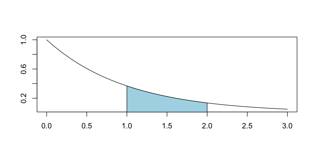
Figure 4.1: \(P(1 \leq X \leq 2)\) for a random variable \(X\) with pdf \(f(x) = e^{-x}\).
Find \(P(1 \le X \le 2)\), which is the shaded area shown in the graph. By definition, \[ P(1\le X \le 2) = \int_1^2 e^{-x}\, dx = -e^{-x}\Bigl|_1^2 = e^{-1} - e^{-2} \approx .233 \]
Find \(P(X \ge 1| X \le 2)\). This is the conditional probability that \(X\) is greater than 1, given that \(X\) is less than or equal to 2. We have \[\begin{align*} P(X \ge 1| X \le 2) &= P( X \ge 1 \cap X \le 2)/P(X \le 2)\\ &=P(1 \le X \le 2)/P(X \le 2)\\ &=\frac{e^{-1} - e^{-2}}{1 - e^{-2}} \approx .269 \end{align*}\]
Let \(X\) have the pdf: \[ f(x) = \begin{cases} 0 & x < 0\\ 1 & 0 \le x \le 1\\ 0 & x \ge 1 \end{cases} \]
\(X\) is called the uniform random variable on the interval \([0,1]\) and realizes the idea of choosing a random number between 0 and 1.
Here are some simple probability computations involving \(X\): \[ \begin{aligned} P(X > 0.3) &= \int_{0.3}^{1}1\,dx = 0.7\\ \\ P(0.2 < X < 0.5) &= \int_{0.2}^{0.5}1\,dx = 0.3 \end{aligned} \]
The cdf for \(X\) is given by: \[ F(x) = \begin{cases} 0 & x < 0\\ x & 0\le x \le 1\\ 1 & x \ge 1 \end{cases} \]
The pdf and cdf of the uniform random variable \(X\) are implemented in R with the functions dunif and punif.
Here are plots of these functions, produced by plot and by choosing a sequence
of x values that cover the interesting range of the pdf and cdf:
x <- seq(-0.5, 1.5, 0.01)
plot(x, dunif(x))
plot(x, punif(x))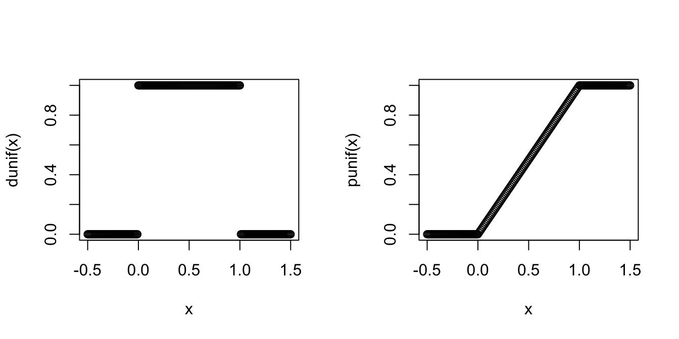
We can produce simulated values of \(X\) with the function runif
and use those to estimate probabilities:
X <- runif(10000)
mean(X > 0.3)
## [1] 0.7041mean(0.2 < X & X < 0.5)## [1] 0.3015Here, we have used the vectorized version of the and operator, &.
It is important to distinguish between the operator & and the operator && when doing simulations, or any time that you are doing logical operations on vectors. If you use && on two vectors, older versions of R ignore all entries except the first, and newer versions return an error!
For example,
c(TRUE, TRUE, TRUE) && c(TRUE, FALSE, FALSE)## Error in c(TRUE, TRUE, TRUE) && c(TRUE, FALSE, FALSE): 'length = 3' in
## coercion to 'logical(1)'But, compare to
c(TRUE, TRUE, TRUE) & c(TRUE, FALSE, FALSE)## [1] TRUE FALSE FALSESuppose \(X\) is a random variable with cdf given by
\[ F(x) = \begin{cases} 0 & x < 0\\ x/2 & 0\le x \le 2\\ 1 & x \ge 2 \end{cases} \]
Find \(P(1 \le X \le 2)\). To do this, we note that \(P(1 \le X \le 2) = F(2) - F(1) = 1 - 1/2 = 1/2\).
Find \(P(X \ge 1/2)\). To do this, we note that \(P(X \ge 1/2) = 1 - F(1/2) = 1 - 1/4 = 3/4\).
To find the pdf associated with \(X\), we take the derivative of \(F\). Since pdfs are only used via integration, it doesn’t matter how we define the pdf at the places where \(F\) is not differentiable. In this case, we set \(f\) equal to \(1/2\) at those places to get \[ f(x) = \begin{cases} 1/2 & 0 \le x \le 2\\ 0& \text{otherwise} \end{cases} \] This example is also a uniform random variable, this time on the interval \([0,2]\).
Let \(X\) and \(Y\) be independent uniform random variables on \([0,1]\). Find the cumulative distribution function \(F_W\) for the random variable \(W\) which is the larger of \(X\) and \(Y\).
In Example 4.7 we saw that both \(X\) and \(Y\) have cdf given by
\[ F(x) = \begin{cases} 0&x < 0\\x&0\le x \le 1\\1&x > 1\end{cases}. \]
Let’s start with the observation that \(W \le w\) exactly when both \(X \le w\) and \(Y \le w\). Therefore,
\[ F_W(w) = P(W \le w) = P(X \le w \text{ and } Y \le w) = P(X \le w)P(Y \le w) = F(w)F(w) = F(w)^2. \]
The middle equality used the multiplication rule for independent events, since \(X\) and \(Y\) are independent. Then,
\[ F_W(w) = F(w)^2 = \begin{cases}0& w < 0\\w^2&0\le w \le 1\\1&w > 1\end{cases} \]
The pdf of \(W\) we compute by differentiating \(F_W(w)\) to get: \[ f_W(w) = \begin{cases} 0 & w < 0\\ 2w & 0\le w \le 1\\ 0 & w > 1 \end{cases} \]
We can confirm this answer by estimating the probability that the maximum of two uniform random variables is less than or equal to 2/3.
We start by taking large samples from two independent uniform distributions, and then we need to take the pairwise maximums of the vectors.
Note that max will not work in this case, because it will simply take the maximum of the entire vector, so we need to use the parallel version pmax.
X <- runif(10000, 0, 1)
Y <- runif(10000, 0, 1)
W <- pmax(X, Y)
mean(W < 2 / 3)
## [1] 0.4444We get that \(P(W < 2/3) \approx\) 0.4444, which is close to the true value \(F_W(2/3) = (2/3)^2 = 4/9\).
Exercise 5.15 in Chapter 5 asks you to estimate the pdf of \(W\) using simulation.
4.2 Expected value
Let \(X\) be a continuous random variable with pdf \(f\).
The expected value of \(X\) is \[ E[X] = \int_{-\infty}^{\infty} x f(x)\, dx \]
Find the expected value of \(X\) when its pdf is given by \(f(x) = e^{-x}\) for \(x > 0\).
We compute \[ E[X] = \int_{-\infty}^{\infty}f(x) dx = \int_0^\infty x e^{-x} \, dx = \left(-xe^{-x} - e^{-x}\right)\Bigr|_0^\infty = 1 \] (Recall: to integrate \(xe^{-x}\) you use integration by parts.)
Find the expected value of the uniform random variable on \([0,1]\). Using integration, we get the exact result: \[ E[X] = \int_0^1 x \cdot 1\, dx = \frac{x^2}{2}\Biggr|_0^1 = \frac{1}{2} \]
Approximating with simulation,
X <- runif(10000)
mean(X)
## [1] 0.495409Observe that the formula for the expected value of a continuous rv is the same as the formula for center of mass. If the area under the pdf \(f(x)\) is cut from a thin sheet of material, the expected value is the point on the \(x\)-axis where this material would balance.
The balance point is at \(X = 1/2\) for the uniform random variable on [0,1], since the pdf describes a square with base \([0,1]\).
For \(X\) with pdf \(f(x) = e^{-x}, x \ge 0\), Figure 4.2 shows \(E[X]=1\) as the balancing point for the shaded region.
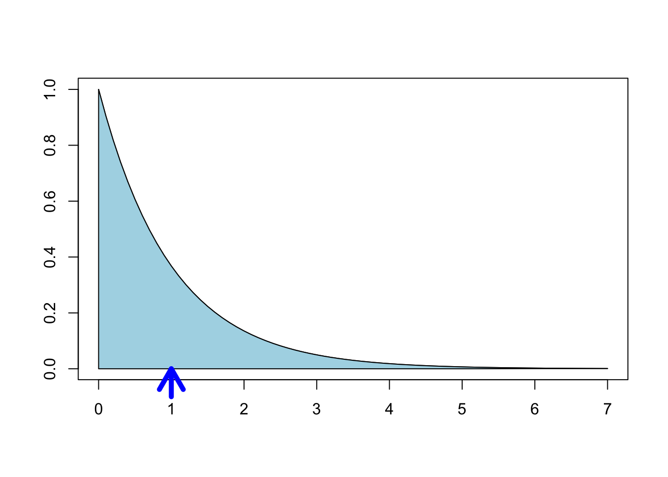
Figure 4.2: The expected value of a distribution is its “balancing point”.
As in the discrete case, we can also define functions of random variables. In order to find the probability density function of a function of a continuous random variable, we can find the cumulative distribution function and take its derivative.
Let \(X\) be a uniform random variable on \([0,1]\). Find the cdf of \(X^2 + 1\).
Let \(Y = X^2 + 1\). Since \(X \in [0,1]\), we must have \(Y \in [1,2]\). Then for \(1 \leq y \leq 2\),
\[ P(Y \le y) = P(X^2 + 1 \le y) = P(X \le \sqrt{y - 1}). \]
Since the cdf of \(X\) is given by \(F(x) = x, \,\, 0 \le x \le 1\), we have
\[ P(Y \le y) = \begin{cases} 0, & y < 1 \\ \sqrt{y - 1}, & 1 \le y \le 2 \\ 1,& y > 2\end{cases} \]
As in the discrete case, we will often be interested in computing expected values of functions of random variables.
Let \(X\) be a continuous random variable and let \(g\) be a function.
\[ E[g(X)] = \int g(x) f(x)\, dx \]
Compute \(E[X^2]\) for \(X\) that has pdf \(f(x) = e^{-x}\), \(x > 0\).
Using integration by parts: \[ E[X^2] = \int_0^\infty x^2 e^{-x}\, dx = \left(-x^2 e^{-x} - 2x e^{-x} - 2 e^{-x}\right)\Bigl|_0^\infty = 2. \]
Let \(X\) be the uniform random variable on \([0,1]\), and let \(Y = 1/X\).
What is \(P(Y < 3)\)? The event \(Y < 3\) is the same as \(1/X < 3\) or \(X > 1/3\), so \(P(Y < 3) = P(X > 1/3) = 2/3\). We can check with simulation:
X <- runif(10000)
Y <- 1 / X
mean(Y < 3)
## [1] 0.6733On the other hand, the expected value of \(Y = 1/X\) is not well behaved. We compute: \[ E[1/X] = \int_0^1 \frac{1}{x} dx = \ln(x)\Bigr|_0^1 = \infty \] Small values of \(X\) are common enough that the huge values of \(1/X\) produced cause the expected value to be infinite. Let’s see what this does to simulations:
X <- runif(100)
mean(1 / X)
## [1] 4.116572X <- runif(10000)
mean(1 / X)## [1] 10.65163X <- runif(1000000)
mean(1 / X)## [1] 22.27425Because the expected value is infinite, the simulations are not approaching a finite number as the size of the simulation increases. The reader is encouraged to try running these simulations multiple times to observe the inconsistency of the results.
Expected value is linear, which we stated as Theorem 3.8 in Chapter 3 for discrete random variables. We repeat it here for any type of random variable.
For random variables \(X\) and \(Y\), and constants \(a\), \(b\), and \(c\):
- \(E[aX + bY] = aE[X] + bE[Y]\).
- \(E[c] = c\).
4.3 Variance and standard deviation
The variance and standard deviation of a continuous random variable play the same role as they do for discrete random variables, that is, they measure the spread of the random variable about its mean. The definitions are unchanged from the discrete case (Definition 3.31), and Theorem 3.9 applies just as well to compute variance. For a random variable \(X\) with expected value \(\mu\):
\[\begin{align*} \text{Var}(X) &= E[(X - \mu)^2] = E[X^2] - E[X]^2 \\ \sigma &= \sqrt{\text{Var}(X)} \end{align*}\]
Compute the variance of \(X\) if the pdf of \(X\) is given by \(f(x) = e^{-x}\), \(x > 0\).
We have already seen that \(E[X] = 1\) and \(E[X^2] = 2\) (Example 4.14). Therefore, the variance of \(X\) is \[ \text{Var}(X) = E[X^2] - E[X]^2 = 2 - 1 = 1. \] The standard deviation \(\sigma(X) = \sqrt{1} = 1\). We interpret the standard deviation \(\sigma\) as a spread around the mean, as shown in Figure 4.3.
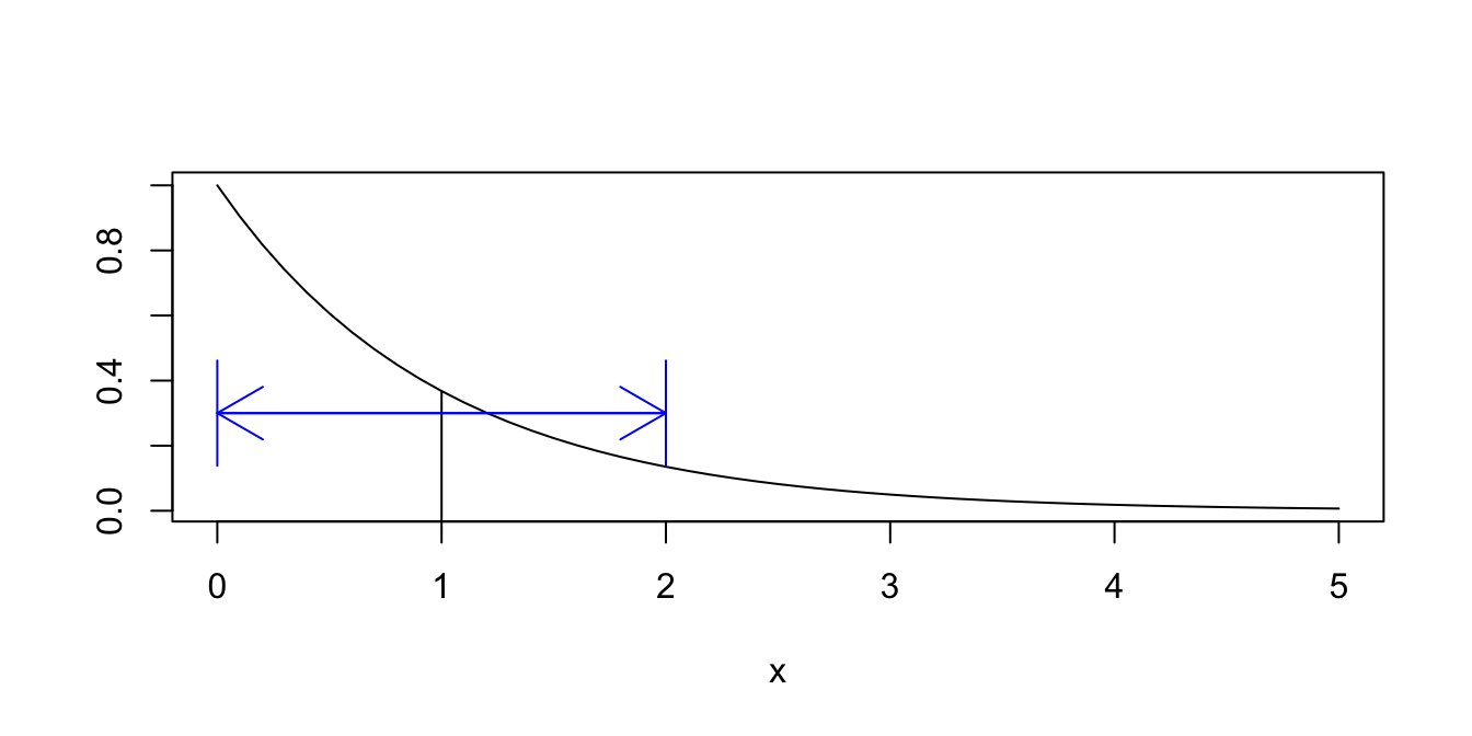
Figure 4.3: One standard deviation above and below the mean \(\mu = 1\).
In Figure 4.3, the mean 1 is marked with a vertical line, and the two arrows extend one standard deviation in each direction from the mean.
Compute the standard deviation of the uniform random variable \(X\) on \([0,1]\). \[ \begin{split} \text{Var}(X) &= E[X^2] - E[X]^2 = \int_0^1x^2 \cdot 1\, dx - \left(\frac{1}{2}\right)^2\\ &= \frac{1}{3} - \frac{1}{4} = \frac{1}{12} \approx 0.083. \end{split} \] So the standard deviation is \(\sigma(X) = \sqrt{1/12} \approx 0.289\). Figure 4.4 shows a one standard deviation spread around the mean of 1/2.
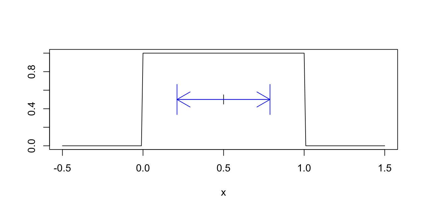
Figure 4.4: One standard deviation above and below the mean \(\mu = 0.5\).
For many distributions, most of the values will lie within one standard deviation of the mean, i.e., within the spread shown in the example pictures. Almost all of the values will lie within two standard deviations of the mean. What do we mean by “almost all”? Well, 85% would be almost all; 15% would not be almost all. This is a very vague rule of thumb. Chebychev’s Theorem is a more precise statement. It says in particular that the probability of being more than two standard deviations away from the mean is at most 25%.
Sometimes, you know that the data you collect will likely fall in a certain range of values. For example, if you are measuring the height in inches of 100 randomly selected adult males, you would be able to guess that your data will very likely lie in the interval 60-84. You can get a rough estimate of the standard deviation by taking the expected range of values and dividing by 6; in this case it would be 24/6 = 4. Here, we are using the heuristic that it is very rare for data to fall more than three standard deviations from the mean. This can be useful as a quick check on your computations.
4.4 Normal random variables
The normal distribution is the most important in statistics. It is often referred to as the bell curve, because its shape resembles a bell:

The importance of the normal distribution stems from the Central Limit Theorem, which implies that many random variables have normal distributions. A little more accurately, the Central Limit Theorem says that random variables which are the sum of many small independent factors are approximately normal.
For example, we might model the heights of adult females with a normal distribution. We imagine that adult height is affected by genetic contributions from generations of parents together with the sum of contributions from food eaten and other environmental factors. This is a reason to try a normal model for heights of adult females, and certainly should not be seen as a theoretical justification of any sort that adult female heights must be normal.
Many measured quantities are commonly modeled with normal distributions. Biometric measurements (height, weight, blood pressure, wingspan) are often nearly normal. Standardized test scores, economic indicators, scientific measurement errors, and variation in manufacturing processes are other examples.
The mathematical definition of the normal distribution begins with the function \(h(x) = e^{-x^2}\), which produces the bell shaped curve shown above, centered at zero and with tails that decay very quickly to zero. By itself, \(h(x) = e^{-x^2}\) is not a distribution since it does not have area 1 underneath the curve. In fact:
\[ \int_{-\infty}^\infty e^{-x^2} dx = \sqrt{\pi} \]
This famous result is known as the Gaussian integral. Its proof is left to the reader in Exercise 4.14. By rescaling, we arrive at an actual pdf given by \(g(x) = \frac{1}{\sqrt{\pi}}e^{-x^2}\). The distribution \(g(x)\) has mean zero and standard deviation \(\frac{1}{\sqrt{2}} \approx 0.707\). The inflection points of \(g(x)\) are also at \(\pm \frac{1}{\sqrt{2}}\) and so rescaling by 2 in the \(x\) direction produces a pdf with standard deviation 1 and inflection points at \(\pm 1\).
The standard normal random variable \(Z\) has probability density function given by \[ f(x) = \frac{1}{\sqrt{2\pi}} e^{-x^2/2}. \] The graph of \(f(x)\) is shown in Figure 4.5.
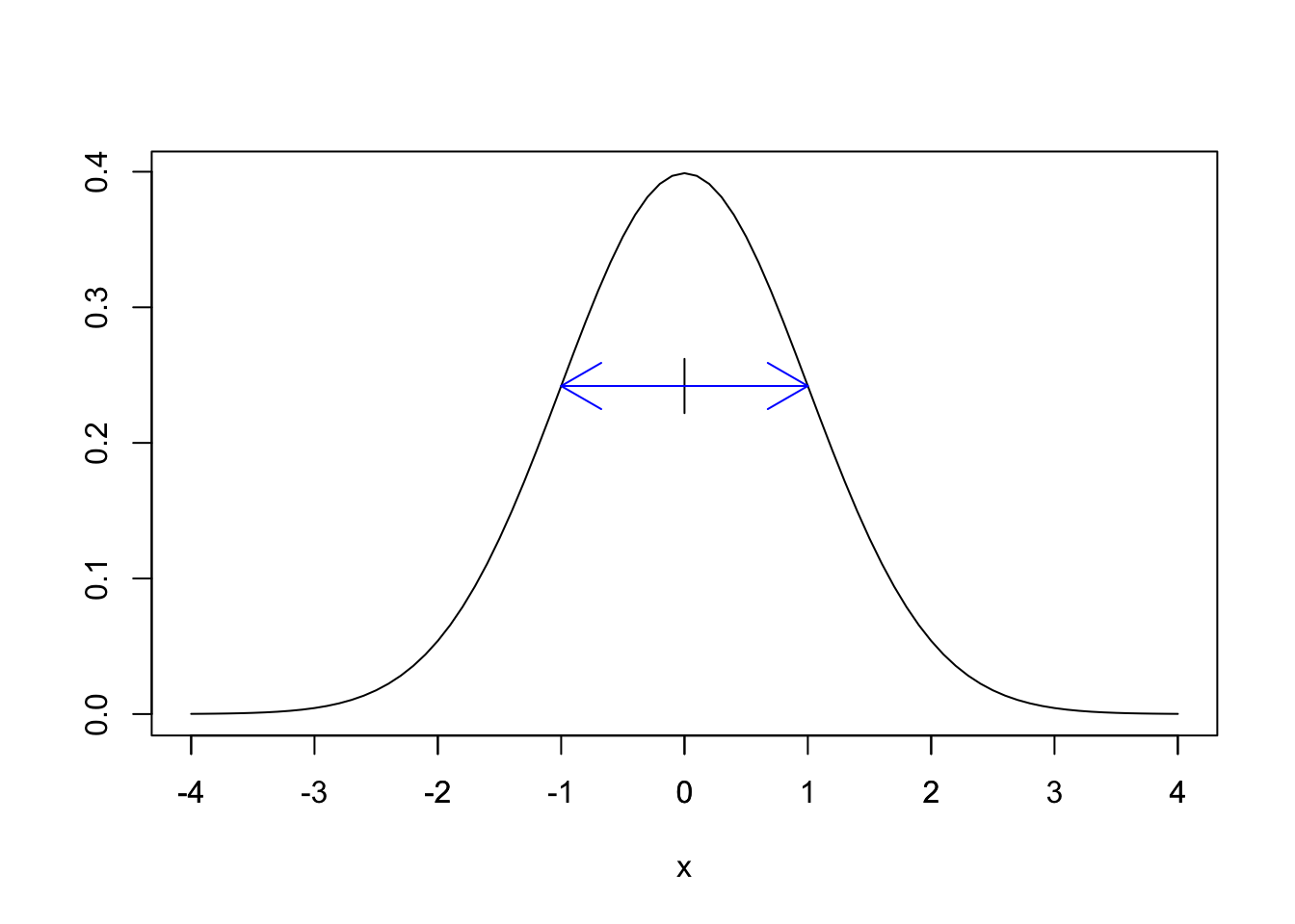
Figure 4.5: The standard normal distribution (with one s.d. shown).
The R function pnorm computes the cdf of the normal distribution,
as pnorm(x) \(= P(Z \leq x)\). Using pnorm, we can compute the probability that \(Z\) lies within 1, 2, and 3 standard deviations of its mean:
- \(P(-1 \leq Z \leq 1) = P(Z \leq 1) - P(Z \leq -1) =\)
pnorm(1) - pnorm(-1)= 0.6826895. - \(P(-2 \leq Z \leq 2) = P(Z \leq 2) - P(Z \leq -2) =\)
pnorm(2) - pnorm(-2)= 0.9544997. - \(P(-3 \leq Z \leq 3) = P(Z \leq 3) - P(Z \leq -3) =\)
pnorm(3) - pnorm(-3)= 0.9973002.
By shifting and rescaling \(Z\), we define the normal random variable with mean \(\mu\) and standard deviation \(\sigma\):
The normal random variable \(X\) with mean \(\mu\) and standard deviation \(\sigma\) is given by \[ X = \sigma Z + \mu. \] We write \(X \sim \text{Norm}(\mu,\sigma)\).
Many books write \(X \sim N(\mu, \sigma^2)\), so that the second parameter in the parenthesis is the variance. We use the standard deviation and the abbreviation Norm to be consistent with R.
The pdf of a normal random variable is given in the following theorem.
Let \(X\) be a normal random variable with parameters \(\sigma\) and \(\mu\). The probability mass function of \(X\) is given by \[ f(x) = \frac {1}{\sigma\sqrt{2\pi}} e^{-\frac{1}{2}\left(\frac{x - \mu}{\sigma}\right)^2} \qquad -\infty < x < \infty \]
The parameter names are the mean \(\mu\) and the standard deviation \(\sigma\).
For any normal random variable, approximately:
- 68% of the normal distribution lies within one standard deviation of the mean.
- 95% lies within two standard deviations of the mean.
- 99.7% lies within three standard deviations of the mean.
This fact is sometimes called the empirical rule.
Figure 4.6 shows examples of normal distributions with fixed mean \(\mu = 0\) and various values of the standard deviation \(\sigma\). Figure 4.7 shows normal distributions with fixed standard deviation \(\sigma = 1\) and various means \(\mu\).
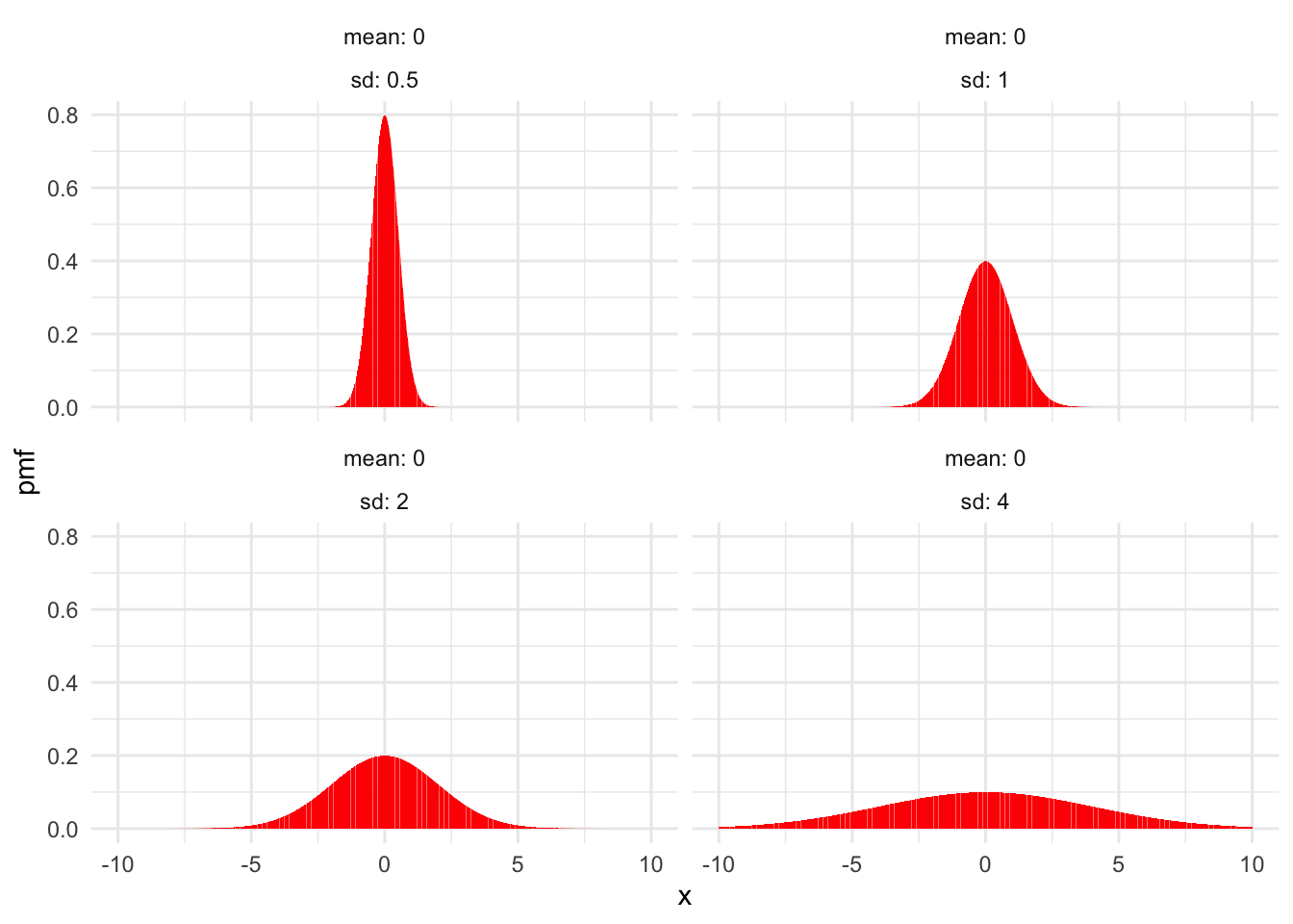
Figure 4.6: Normal distributions with \(\mu = 0\) and various values of \(\sigma\).
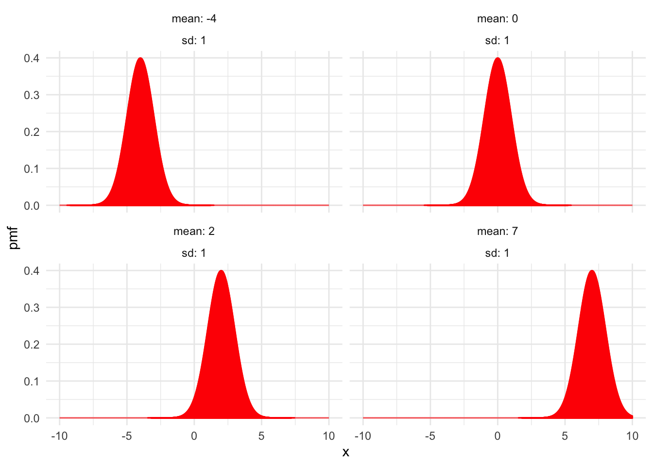
Figure 4.7: Normal distributions with \(\sigma = 1\) and various values of \(\mu\).
4.4.1 Computations with normal random variables
R has built-in functions for working with normal distributions and normal random variables. The root name for these functions is norm, and as with other distributions the prefixes d, p, and r specify the pdf, cdf, or random sampling.
We also introduce the q prefix here, which indicates the inverse of the cdf function.
The q prefix is available for all random variables supported by R, but we will rarely use it for anything except normal rvs.
If \(X \sim \text{Norm}(\mu,\sigma)\):
dnorm(x, mu, sigma)gives the height of the pdf at \(x\).pnorm(x, mu, sigma)gives \(P(X \leq x)\), the cdf.qnorm(p, mu, sigma)gives the value of \(x\) so that \(P(X \leq x) = p\), the inverse cdf.rnorm(N, mu, sigma)simulates \(N\) random values of \(X\).
Here are some simple examples:
Let \(X \sim {\rm Norm}(\mu = 3, \sigma = 2)\). Find \(P(X \le 4)\) and \(P(0 \le X \le 5)\).
pnorm(4, mean = 3, sd = 2)## [1] 0.6914625pnorm(5, 3, 2) - pnorm(0, 3, 2)## [1] 0.7745375Let \(X \sim {\rm Norm}(100,30)\).
Find the value of \(q\) such that \(P(X \le q) = 0.75\). One approach is to try various choices of \(q\) until discovering that pnorm(120,100,30) is close to 0.75.
However, the purpose of the qnorm function is to answer this exact question:
qnorm(0.75, 100, 30)## [1] 120.2347The length of dog pregnancies from conception to birth varies according to a distribution that is approximately normal with mean 63 days and standard deviation 2 days.
- What percentage of dog pregnancies last 60 days or fewer?
- What percentage of dog pregnancies last 67 days or more?
- What range covers the shortest 90% of dog pregnancies?
- What is the narrowest range of times that covers 90% of dog pregnancies?
We let \(X\) be the random variable which is the length of a dog pregnancy. We model \(X \sim \text{Norm}(63,2)\). Then parts (a) and (b) ask for \(P(X \leq 60)\) and \(P(X \geq 67)\) and we can compute these with pnorm as follows:
pnorm(60, 63, 2)## [1] 0.06680721 - pnorm(67, 63, 2)## [1] 0.02275013For part (c), we want \(x\) so that \(P(X \leq x) = 0.90\). This is qnorm(0.90,63,2)=65.6, so 90% of dog pregnancies are shorter than 65.6 days.
For part (d), we need to use the fact that the pdfs of normal random variables are symmetric about their mean, and decreasing away from the mean. So, if we want the shortest interval that contains 90% of dog pregnancies, it should be centered at the mean with 5% of pregnancies to the left of the interval, and 5% of the pregnancies to the right of the interval. We get an interval of the form [qnorm(0.05, 63, 2), qnorm(0.95, 63, 2)], or approximately [59.7, 66.3].
Let \(Z\) be a standard normal random variable. Find the mean and standard deviation of the variable \(e^Z\).
We solve this with simulation:
Z <- rnorm(100000, 0, 1)
mean(exp(Z))
## [1] 1.648321sd(exp(Z))## [1] 2.149228The mean of \(e^Z\) is approximately 1.6, and the standard deviation is approximately 2.1. Note that even with 100,000 simulated values, these answers are not particularly accurate because on rare occasions \(e^Z\) takes on very large values.
Suppose you are picking seven women at random from a university to form a starting line-up in an ultimate frisbee game. Assume that women’s heights at this university are normally distributed with mean 64.5 inches (5 foot, 4.5 inches) and standard deviation 2.25 inches. What is the probability that 3 or more of the women are 68 inches (5 foot, 8 inches) or taller?
To do this, we first determine the probability that a single randomly selected woman is 68 inches or taller.
Let \(X\) be a normal random variable with mean 64 and standard deviation 2.25. We compute \(P(X \ge 68)\) using pnorm:
pnorm(68, 65, 2.25, lower.tail = FALSE)## [1] 0.09121122Now, we need to compute the probability that 3 or more of the 7 women are 68 inches or taller. Since the population of all women at a university is much larger than 7, the number of women in the starting line-up who are 68 inches or taller is binomial with \(n = 7\) and \(p = 0.09121122\), which we computed in the previous step. We compute the probability that at least 3 are 68 inches as
sum(dbinom(3:7, 7, 0.09121122))## [1] 0.02004754So, there is about a 2% chance that at least three will be 68 inches or taller.
How likely is it that the team has no players who are 68 inches or taller?
dbinom(0, 7, 0.09121122)## [1] 0.5119655According to our model, this happens about 50% of the time. None of the 2019 national champion UC San Diego Psychos were 68 inches or taller, although it is unlikely that ultimate frisbee players are drawn randomly from the population of women.
Throwing a dart at a dartboard with the bullseye at the origin, model the location of the dart with independent coordinates \(X \sim \text{Norm}(0,3)\) and \(Y \sim \text{Norm}(0,3)\) (both in inches). What is the expected distance from the bullseye?
The distance from the bullseye is given by the Euclidean distance formula \(d = \sqrt{X^2+ Y^2}\). We simulate the \(X\) and \(Y\) random variables and then compute the mean of \(d\):
X <- rnorm(10000, 0, 3)
Y <- rnorm(10000, 0, 3)
d <- sqrt(X^2 + Y^2)
mean(d)
## [1] 3.759785We expect the dart to land about 3.8 inches from the bullseye, on average.
4.4.2 Normal approximation to the binomial
The value of a binomial random variable is the sum of independent factors: the Bernoulli trials. A special case of the Central Limit Theorem is that a binomial random variable can be well approximated by a normal random variable when the number of trials is large.
First, we need to understand the standard deviation of a binomial random variable.
Let \(X \sim \text{Binom}(n,p)\). The variance and standard deviation of \(X\) are given by: \[\begin{align} \text{Var}(X) &= np(1-p)\\ \sigma(X) &= \sqrt{np(1-p)} \end{align}\]
The proof of this theorem was given in Example 3.35. There is also an instructive proof that is similar to the proof of Theorem 3.3, except that we take the derivative of the binomial theorem two times and compute \(E[X(X-1)]\). The result follows from \(E[X^2] = E[X(X-1)] + E[X]\) and Theorem 3.9.
Now the binomial rv \(X\) can be approximated by a random normal variable with the same mean and standard deviation as \(X\):
Fix \(p\). For large \(n\), the binomial random variable \(X \sim \text{Binom}(n,p)\) is approximately normal with mean \(\mu = np\) and standard deviation \(\sigma = \sqrt{np(1-p)}\).
The size of \(n\) required to make the normal approximation accurate depends on the accuracy required and also depends on \(p\). Binomial distributions with \(p\) close to 0 or 1 are not as well approximated by the normal distribution as those with \(p\) near 1/2.
This normal approximation was traditionally used to work with binomial random variables, since calculating the binomial distribution exactly requires quite a bit of computation. Probabilities for the normal distribution were readily available in tables, and so were easier to use. With R, the pbinom function makes it easy to work with binomial pmfs directly.
Let \(X \sim \text{Binom}(300,0.46)\). Compute \(P(X > 150)\).
Computing exactly, \(P(X > 150) =\) 1 - pbinom(150,300,0.46) = 0.0740.
To use the normal approximation, we calculate that \(X\) has mean \(300 \cdot 0.46 = 138\) and standard deviation
\(\sqrt{300\cdot0.46\cdot0.54} \approx 8.63\). Then \(P(X > 150) \approx\) 1 - pnorm(150,138,8.63) = 0.0822.
As an improvement, notice that the continuous normal variable can take values in between 150 and 151, but the discrete binomial variable cannot. To account for this, we use a continuity correction and assign each integer value of the binomial variable to the one-unit wide interval centered at that integer. Then 150 corresponds to the interval (145.5,150.5) and 151 corresponds to the interval (150.5,151.5). To approximate \(X > 150\), we
want our normal random variable to be larger than 150.5. The normal approximation with continuity correction gives
\(P(X > 150) \approx\) 1 - pnorm(150.5,138,8.63) = 0.0737, much closer to the actual value of 0.0740.
4.5 Uniform and exponential random variables
4.5.1 Uniform random variables
Uniform random variables may be discrete or continuous.
A discrete uniform variable may take any one of finitely many values, all equally likely. The classic example is the die roll, which is uniform on the numbers 1,2,3,4,5,6. Another example is a coin flip, where we assign 1 to heads and 0 to tails. Unlike most other named random variables, R has no special functions for working with discrete uniform variables. Instead, we use sample to simulate these.
A continuous uniform random variable \(X\) on the interval \([a,b]\) has pdf given by \[ f(x) = \begin{cases} \frac{1}{b -a} & a \le x \le b\\0&{\rm otherwise} \end{cases} \] The graph of \(f(x)\) is shown in Figure 4.8.
![PDF of a continuous uniform random variable on $[a,b]$.](04-continuousrvs_files/figure-html/crvunifplot-1.png)
Figure 4.8: PDF of a continuous uniform random variable on \([a,b]\).
A continuous uniform rv \(X\) is characterized by the property that for any interval \(I \subset [a,b]\), the probability \(P(X \in I)\) depends only on the length of \(I\). We write \(X \sim \text{Unif}(a,b)\) if \(X\) is continuous uniform on the interval \([a,b]\).
One example of a random variable that could be modeled by a continuous uniform random variable is a round-off error in measurements. Say we measure height and record only feet and inches. It is a reasonable first approximation that the error associated with rounding to the nearest inch is uniform on the interval \([-1/2,1/2]\). There may be other sources of measurement error which might not be well modeled by a uniform random variable, but the round-off is uniform.
Another example is related to the Poisson process. If you observe a Poisson process after some length of time \(T\) and see that exactly one event has occurred, then the time that the event occurred in the interval \([0, T]\) is uniformly distributed.
A random real number is chosen uniformly in the interval 0 to 10. What is the probability that it is bigger than 7, given that it is bigger than 6?
Let \(X \sim \text{Unif}(0,10)\) be the random real number. Then \[ P(X > 7\ |\ X > 6) = \frac{P(X > 7 \cap X > 6)}{P(X > 6)} = \frac{P(X > 7)}{P(X > 6)} =\frac{3/10}{4/10} = \frac{3}{4}. \]
Alternately, we can compute with the punif function, which gives the cdf of a uniform random variable.
(1 - punif(7, 0, 10)) / (1 - punif(6, 0, 10))## [1] 0.75The conditional density of a uniform over the interval \([a,b]\) given that it is in the subset \([c,d]\) is uniformly distributed on the interval \([c,d]\). Applying that fact to Example 4.28, we know that \(X\) given \(X > 6\) is uniform on the interval \([6, 10]\). Therefore, the probability that \(X\) is larger than 7 is simply 3/4. Note that this only works for uniform random variables! For other random variables, you need to compute conditional probabilities as in Example 4.28.
We finish this section with a computation of the mean and variance of a uniform random variable \(X\). Not surprisingly, the mean is exactly halfway along the interval of possible values for \(X\).
For \(X \sim \text{Unif}(a,b)\), the expected value of \(X\) is \[ E[X] = \frac{b + a}{2}\] and the variance is \[ \text{Var}(X) = \frac{(b - a)^2}{12} \]
We compute the mean of \(X\) as follows: \[\begin{align*} E[X] &= \int_a^b \frac{x}{b-a}\, dx = \left.\frac{x^2}{2(b - a)}\right|_{x = a}^{x = b}\\ &=\frac{b^2}{2(b-a)} - \frac{a^2}{2(b-a)} = \frac{(b - a)(b + a)}{2(b - a)}\\ &=\frac{a+b}{2}. \end{align*}\]
For the variance, first calculate \(E[X^2] = \int_a^b \frac{x^2}{b-a}dx\). Then \[ \text{Var}(X) = E[X^2] - E[X]^2 = E[X^2] - \left(\frac{a+b}{2}\right)^2. \] Working the integral and simplifying \(\text{Var}(X)\) is left as Exercise 4.20.
4.5.2 Exponential random variables
An exponential random variable \(X\) with rate \(\lambda\) has pdf \[ f(x) = \lambda e^{-\lambda x}, \qquad x > 0 \]
We write \(X \sim \text{Exp}(\lambda)\). Figure 4.9 shows the graph of \(f(x)\) for various values of the rate \(\lambda\).
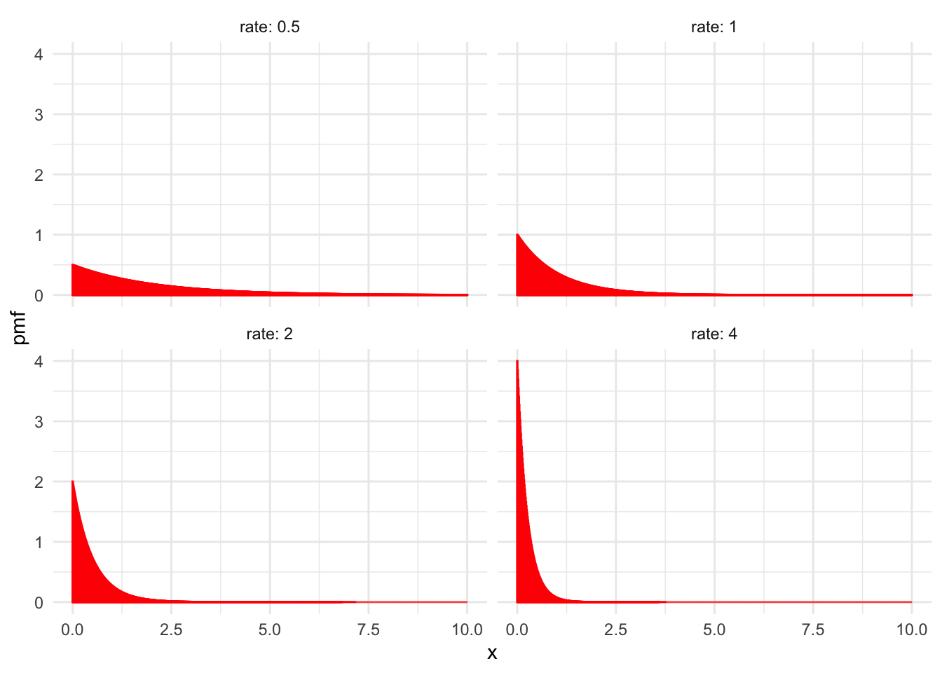
Figure 4.9: Exponential distributions with various values of \(\lambda\).
Exponential random variables measure the waiting time until the first event occurs in a Poisson process, see Section 3.6.1. The waiting time until an electronic component fails could be exponential. In a store, the time between customers could be modeled by an exponential random variable by starting the Poisson process at the moment the first customer enters. Observe in Figure 4.9 that the higher the rate, the smaller \(X\) will be. This is because we generally wait less time for events that occur more frequently.
The exponential distribution is a skew distribution, which means it is not symmetric. Because it has a long tail on the right, we say it has right skew.
Let \(X \sim \text{Exp}(\lambda)\) be an exponential random variable with rate \(\lambda\). Then the mean and variance of \(X\) are: \[\begin{align} E[X] &= \frac{1}{\lambda}\\ \text{Var}(X) &= \frac{1}{\lambda^2} \end{align}\]
We compute the mean of an exponential random variable with rate \(\lambda\) using integration by parts as follows: \[\begin{align*} E[X]&=\int_{-\infty}^\infty x f(x)\, dx\\ &=\int_0^\infty x \lambda e^{-\lambda x} + \int_{-\infty}^0 x \cdot 0 \, dx\\ &= -xe^{-\lambda x} - \frac {1}{\lambda} e^{-\lambda x}\big|_{x = 0}^{x = \infty}\\ & = \frac {1}{\lambda} \end{align*}\]
For the variance, we compute the rather challenging integral: \[ E[X^2] = \int_0^\infty x^2 \lambda e^{-\lambda x} dx = \frac{2}{\lambda^2} \] Then \[ \text{Var}(X) = E[X^2] - E[X]^2 = \frac{2}{\lambda^2} - \left(\frac{1}{\lambda}\right)^2 = \frac{1}{\lambda^2}. \]
When watching the Taurids meteor shower, meteors arrive at a rate of five per hour. How long do you expect to wait for the first meteor? How long should you wait to have a 95% change of seeing a meteor?
Here, \(X\) is the length of time before the first meteor. We model the meteors as a Poisson process with rate \(\lambda = 5\) (and time in hours). Then \(E[X] = \frac{1}{5} = 0.2\) hours, or 12 minutes.
For a 95% chance, we are interested in finding \(x\) so that \(P(X < x) = 0.95\). One way to approach this is by playing with values of \(x\) in the R function pexp(x,5). Some effort will yield pexp(0.6,5) = 0.95, so that we should plan on waiting 0.6 hours, or 36 minutes to be 95% sure of seeing a meteor.
A more straightforward approach is to use the inverse cdf function qexp, which gives
qexp(0.95, 5)## [1] 0.5991465and the exact waiting time of 0.599 hours.
The memoryless property of exponential random variables is the equation \[ P(X > s + t\,|\,X > s) = P(X > t) \] for any \(s,t > 0\). It helps to interpret this equation in the context of a Poisson process, where \(X\) measures waiting time for some event. The left-hand side of the equation is the probability that we wait \(t\) units longer, given that we have already waited \(s\) units. The right-hand side is the probability that we wait \(t\) units, from the beginning. Because these two probabilities are the same, it means that waiting \(s\) units has gotten us no closer to the occurrence of the event. The Poisson process has no memory that you have “already waited” \(s\) units.
We prove the memoryless property here by computing the probabilities involved. The cdf of an exponential random variable with rate \(\lambda\) is given by \[ F(x) = \int_{0}^\infty e^{-\lambda x} dx = 1 - e^{-\lambda x} \] for \(x > 0\). Then \(P(X > x) = 1 - F(x) = e^{-\lambda x}\), and \[\begin{align*} P(X > s + t\,|\,X > s) &= \frac{P(X > s + t\,\cap\,X > s)}{P(X > s)} \\ &=\frac{P(X > s + t)}{P(X > s)}\\ &=e^{-\lambda(s + t)}/e^{-\lambda s}\\ &=e^{-\lambda t}\\ &=P(X > t) \end{align*}\]
4.6 Summary
This chapter and Chapter 3 introduced the notion of a random variable, and the associated notion of a probability distribution. For any random variable, we might be interested in answering probability questions either exactly or through simulation. Usually, these questions involve knowledge of the probability distribution. For some commonly occurring types of random variable, the probability distribution functions are well understood.
The following table provides a quick reference for random variables introduced so far, together with pmf/pdf, expected value, variance and root R function.
| RV | PMF/PDF | Range | Mean | Variance | R Root |
|---|---|---|---|---|---|
| Binomial | \({\binom{n}{x}} p^x(1 - p)^{n - x}\) | \(0\le x \le n\) | \(np\) | \(np(1 - p)\) | binom |
| Geometric | \(p(1-p)^{x}\) | \(x \ge 0\) | \(\frac{1-p}{p}\) | \(\frac{1-p}{p^2}\) | geom |
| Poisson | \(\frac {1}{x!} \lambda^x e^{-\lambda}\) | \(x \ge 0\) | \(\lambda\) | \(\lambda\) | pois |
| Hypergeometric | \(\frac{{\binom{m}{x}} {\binom{n}{k-x}}}{{\binom{m+n}{k}}}\) | \(x = 0,\ldots,k\) | \(kp\) | \(kp(1-p)\frac{m + n - k}{m + n - 1}\) | hyper |
| Negative Binomial | \(\binom{x + n - 1}{x} p^n (1 - p)^x\) | \(x \ge 0\) | \(n\frac{1-p}p\) | \(n\frac{1-p}{p^2}\) | nbinom |
| Uniform | \(\frac{1}{b - a}\) | \(a \le x \le b\) | \(\frac{a + b}{2}\) | \(\frac{(b - a)^2}{12}\) | unif |
| Exponential | \(\lambda e^{-\lambda x}\) | \(x \ge 0\) | \(1/\lambda\) | \(1/\lambda^2\) | exp |
| Normal | \(\frac 1{\sigma\sqrt{2\pi}} e^{-(x - \mu)^2/(2\sigma^2)}\) | \(-\infty < x < \infty\) | \(\mu\) | \(\sigma^2\) | norm |
When modeling a count of something, you often need to choose between binomial, geometric, and Poisson. The binomial and geometric random variables both come from Bernoulli trials, where there is a sequence of individual trials each resulting in success or failure. In the Poisson process, events are spread over a time interval, and appear at random.
The normal random variable is a good starting point for continuous measurements that have a central value and become less common away from that mean. Exponential variables show up when waiting for events to occur. Continuous uniform variables sometimes occur as the location of an event in time or space, when the event is known to have happened on some fixed interval.
R provides these random variables (and many more!) through a set of four functions for each known distribution.
The four functions are determined by a prefix, which can be p, d, r, or q. The root determines which distribution we are talking about.
Each distribution function takes a single argument first, determined by the prefix, and then some number of parameters, determined by the root. The general form of a distribution function in R is:
[prefix][root] ( argument, parameter1, parameter2, ..)
The available prefixes are:
p- compute the cumulative distribution function \(P(X < x)\), and the argument is \(x\).
d- compute the pdf or pmf \(f\). The value is \(f(x)\), and the argument is \(x\). In the discrete case, this is the probability \(P(X = x)\).
r- sample from the rv. The argument is \(N\), the number of samples to take.
q- quantile function, the inverse cdf. This computes \(x\) so that \(P(X < x) = q\), and the argument is \(q\).
The distributions we have introduced so far, with their parameters, are:
binom- binomial, parameters are \(n\), number of trials and \(p\), probability of success.
geom- geometric, parameter is \(p\), probability of success.
pois- Poisson, parameter is \(\lambda\), the rate at which events occur, or the mean number of events over the time interval.
nbinom-
negative binomial, parameters are
sizewhich is the number of successes, andprob. hyper- hypergeometric with parameters \(m\), number of white balls, \(n\), number of black balls, \(k\), number of balls drawn without replacement.
unif- uniform, parameters are \(a,b\).
norm- normal, parameters are \(\mu\), the mean, and \(\sigma\), the standard deviation.
exp- exponential, parameter is \(\lambda\), the rate.
There will be many more distributions to come, and the four prefixes work the same way for all of them.
Exercises
Exercises 4.1 – 4.5 require material through Section 4.1.
Let \(X\) be a random variable with pdf given by \(f(x) = 2x\) for \(0\le x \le 1\) and \(f(x) = 0\) otherwise.
- Find \(P(X \ge 1/2)\).
- Find \(P(X \ge 1/2| X \ge 1/4)\).
Let \(X\) be a random variable with pdf \[ f(x) = \begin{cases} Cx^2 & 0 \le x \le 1 \\ C(2 - x)^2 & 1 \le x \le 2 \end{cases} \] Find \(C\).
For each of the following functions, decide whether the function is a valid pdf, a valid cdf or neither.
- \(h(x) = \begin{cases} 1&0\le x \le 2\\-1&2\le x\le 3\\0&{\rm {otherwise}} \end{cases}\)
- \(h(x) = \sin(x) + 1\)
- \(h(x) = \begin{cases} 1 - e^{-x^2}& x\ge 0\\0& x< 0\end{cases}\)
- \(h(x) = \begin{cases} 2xe^{-x^2}&x\ge 0\\0&x < 0\end{cases}\)
Provide an example of a pdf \(f\) for a random variable \(X\) such that there exists an \(x\) for which \(f(x) > 1\). Is it possible to have \(f(x) > 1\) for all values of \(x\)?
Is there a function which is both a valid pdf and a valid cdf? If so, give an example. If not, explain why not.
Exercises 4.6 – 4.8 require material through Section 4.3.
Let \(X\) be a random variable with pdf \(f(x) = 3(1 - x)^2\) when \(0\le x \le 1\), and \(f(x) = 0\) otherwise.
- Verify that \(f\) is a valid pdf.
- Find the mean and variance of \(X\).
- Find \(P(X \le 1/2)\).
- Find \(P(X \le 1/2\ |\ X \ge 1/4)\).
If \(\text{Var}(X) = 3\), what is \(\text{Var}(2X + 1)\)?
Let \(X\) be a random variable whose pdf is given by the plot in Figure 4.10. Assume that the pdf is zero outside of the interval given in the plot.
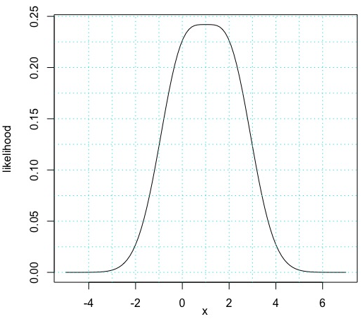
Figure 4.10: PDF of X
- Estimate the mean of \(X\).
- Estimate the standard deviation of \(X\).
- For which \(a\) is \(P(a \le X \le a + 2)\) maximized?
- Estimate \(P(0 \le X \le 2)\).
Exercises 4.9 – 4.14 require material through Section 4.4.
Compare the pdfs of three normal random variables, one with mean 1 and standard deviation 1, one with mean 1 and standard deviation 10, and one with mean -4 and standard deviation 1.
Let \(X\) be a normal rv with mean 1 and standard deviation 2.
- Find \(P(a \le X \le a + 2)\) when \(a = 3\).
- Sketch the graph of the pdf of \(X\), and indicate the region that corresponds to your answer in the previous part.
- Find the value of \(a\) such that \(P(a \le X \le a + 2)\) is the largest.
Suppose that scores on an exam are normally distributed with mean 80 and standard deviation 5, and that scores are not rounded.
- What is the probability that a student scores higher than 85 on the exam?
- Assume that exam scores are independent and that 10 students take the exam. What is the probability that 4 or more students score 85 or higher on the exam?
Climbing rope will break if pulled hard enough. Experiments show that 10.5 mm dynamic nylon rope has a mean breaking point of 5036 lbs with a standard deviation of 122 lbs. Assume breaking points of rope are normally distributed.
- Sketch the distribution of breaking points for this rope.
- What proportion of ropes will break with 5000 lbs of load?
- At what load will 95% of all ropes break?
In this exercise, we verify Theorem 3.10 in a special case. Let \(X\) be normal with mean 0 and standard deviation 2, and let \(Y\) be normal with mean 0 and standard deviation 1. Assume \(X\) and \(Y\) are independent. Use simulation to estimate the variance of \(X + 3Y\), and compare to \(1^2 \times 4 + 3^2 \times 1\).
There is no elementary antiderivative for the function \(e^{x^2}\). However, the Gaussian integral \(\int_{-\infty}^\infty e^{-x^2} dx\) can be computed exactly. Begin with the following: \[ \left(\int_{-\infty}^\infty e^{-x^2} dx\right)^2 = \int_{-\infty}^{\infty} e^{-x^2}\,dx \int_{-\infty}^{\infty} e^{-y^2}\,dy = \int_{-\infty}^{\infty} \int_{-\infty}^{\infty} e^{-(x^2+y^2)}\, dx\,dy \] Now switch to polar coordinates and show that the Gaussian integral is equal to \(\sqrt{\pi}\)
Exercises 4.15 – 4.28 require material through Section 4.5.
Plot the pdf and cdf of a uniform random variable on the interval \([0,1]\).
Compare the cdf and pdf of an exponential random variable with rate \(\lambda = 2\) with the cdf and pdf of an exponential rv with rate 1/2. (If you wish to read ahead in Chapter 7, you can learn how to put plots on the same axes, with different colors.)
Let \(X\) be an exponential rv with rate \(\lambda = 1/4\).
- What is the mean of \(X\)?
- Find the value of \(a\) such that \(P(a \le X \le a + 1)\) is maximized. Is the mean contained in the interval \([a, a+1]\)?
Suppose the time (in seconds) it takes your professor to set up their computer to start class is uniformly distributed on the interval \([0, 30]\). Suppose also that it takes you 5 seconds to send your mom a nice, quick text that you are thinking of her. You only text her if you can complete it during the time your professor is setting up their computer. If you try to text your mom every day in class, what is the probability that she will get a text on 3 consecutive days?
Suppose the time to failure (in years) for a particular component is distributed as an exponential random variable with rate \(\lambda = 1/5\). For better performance, the system has two components installed, and the system will work as long as either component is functional. Assume the time to failure for the two components is independent. What is the probability that the system will fail before 10 years have passed?
Verify that a uniform random variable on the interval \([a,b]\) has variance given by \(\sigma^2 = \frac{(b - a)^2}{12}\).
Let \(X\) be an exponential random variable with rate \(\lambda\). If \(a\) and \(b\) are positive numbers, then \[ P(X > a + b\ |\ X > b) = P(X > a) \]
- Explain why this is called the memoryless property.
- Show that for an exponential rv \(X\) with rate \(\lambda\), \(P(X > a) = e^{-a\lambda}\).
- Use the result in (b) to prove the memoryless property for exponential random variables.
For each of the following descriptions of a random variable, indicate whether it can best be modeled by binomial, geometric, Poisson, uniform, exponential, or normal. Answer the associated questions. Note that not all of the experiments yield random variables that are exactly of the type listed above, but we are asking about reasonable modeling.
- Let \(Y\) be the random variable that counts the number of sixes which occur when a die is tossed 10 times. What type of random variable is \(Y\)? What is \(P(Y=3)\)? What is the expected number of sixes? What is \({\rm Var}(Y)\)?
- Let \(U\) be the random variable which counts the number of accidents which occur at an intersection in one week. What type of random variable is \(U\)? Suppose that, on average, 2 accidents occur per week. Find \(P(U=2)\), \(E(U)\) and \({\rm Var}(U)\).
- Suppose a stop light has a red light that lasts for 60 seconds, a green light that lasts for 30 seconds, and a yellow light that lasts for 5 seconds. When you first observe the stop light, it is red. Let \(X\) denote the time until the light turns green. What type of rv would be used to model \(X\)? What is its mean?
- Customers arrive at a teller’s window at a uniform rate of 5 per hour. Let \(X\) be the length in minutes of time that the teller has to wait until they see their first customer after starting their shift. What type of rv is \(X\)? What is its mean? Find the probability that the teller waits less than 10 minutes for their first customer.
- A coin is tossed until a head is observed. Let \(X\) denote the total number of tails observed during the experiment. What type of rv is \(X\)? What is its mean? Find \(P(X \le 3)\).
- Let \(X\) be the recorded body temperature of a healthy adult in degrees Fahrenheit. What type of rv is \(X\)? Estimate its mean and standard deviation, based on your knowledge of body temperatures.
Suppose you turn on a soccer game and see that the score is 1-0 after 30 minutes of play. Let \(X\) denote the time (in minutes from the start of the game) that the goal was scored. What type of rv is \(X\)? What is its mean?
Let \(X_1, X_2, X_3\) be independent uniform random variables on the interval \([0,1]\). Find the cdf of the random variable \(Z\) which is the maximum of \(X_1, X_2\) and \(X_3\). (Hint: the event \(Z \le z\) is the same as the event \((X_1 \le z) \cap (X_2 \le z) \cap (X_3 \le z)\), and \(F(z) = P(Z \le z)\).)
There exist naturally occurring random variables that are neither discrete nor continuous. Suppose a group of people is waiting for one more person to arrive before starting a meeting. Suppose that the arrival time of the person is exponential with mean 4 minutes, and that the meeting will start either when the person arrives, or after 5 minutes, whichever comes first. Let \(X\) denote the length of time the group waits before starting the meeting.
- Find \(P(0 \le X \le 4)\).
- Find \(P(X = 5)\).
Suppose you pick 4 numbers \(x_1, \ldots, x_4\) uniformly in the interval \([0, 1]\) and you create four intervals of length 1/2 centered at the \(x_i\); namely, \([x_i - 1/4, x_i + 1/4]\). Note that these intervals need not be contained in \([0, 1]\).
Estimate via simulation the probability that the union of the 4 intervals is an interval of length at least 1.23
Suppose that you have two infinite, horizontal parallel lines that are one unit apart. You drop a needle of length 1/2 so that its center between the two lines is uniform on \([0, 1]\), and the angle that the needle forms relative to the parallel lines is uniform on \([0, \pi]\).
Estimate the probability that the needle touches one of the parallel lines, and confirm that your answer is approximately \(1/\pi\).
This problem was reported to be a Google interview question. Suppose you have a stick of length one meter. You randomly select two points on the stick, and break the stick at those two places. Estimate the probability that the resulting three pieces of stick can be used to form a triangle.
This problem is a special case of the arc covering problem, which asks the probability that \(n\) randomly placed arcs of length \(a\) cover a circle of circumference 1, which was solved by Stevens in 1939. For general \(a\), we would need to reformulate the problem to be equivalent to the arc question.↩︎