Probability, Statistics, and Data: A Fresh Approach Using R

Chapter 13 Multiple Regression

This chapter deals with multiple regression, where a single numeric response variable depends on multiple explanatory variables. There is a natural tension between explaining the response variable well and keeping the model simple. Our main purpose will be to understand this tension and find a balance between the two competing goals.

13.1 Two explanatory variables

We consider housing sales data from King County, WA, which includes the city of Seattle. The data set houses in the fosdata package contains a record of every house sold in King County from May 2014 through May 2015. For each house, the data includes the sale price along with many variables describing the house and its location.

Our goal is to model the sale price on the other variables. There are many variables that we could use to do this, but in this section we will only consider two of them; namely, the square footage in the house (sqft_living) and the size of the lot (sqft_lot). To keep the size of the problem small, we restrict to the urban ZIP code 98115.

houses_98115 <- fosdata::houses %>%
  filter(zipcode == "98115") %>%
  select(price, sqft_living, sqft_lot)

There are now 583 observations. We start by doing some summary statistics and visualizations.

summary(houses_98115)

##      price          sqft_living      sqft_lot    
##  Min.   : 200000   Min.   : 620   Min.   :  864  
##  1st Qu.: 456750   1st Qu.:1270   1st Qu.: 4080  
##  Median : 567000   Median :1710   Median : 5300  
##  Mean   : 619900   Mean   :1835   Mean   : 5444  
##  3rd Qu.: 719000   3rd Qu.:2285   3rd Qu.: 6380  
##  Max.   :2300000   Max.   :5770   Max.   :30122

It appears that the variables may be right-skewed. Let’s compute the skewness:

apply(houses_98115, 2, e1071::skewness)

##       price sqft_living    sqft_lot 
##   2.0482534   0.9114968   2.9309820

The variables price and sqft_lot are right-skewed and the variable sqft_living is moderately right-skewed. Let’s look at histograms.

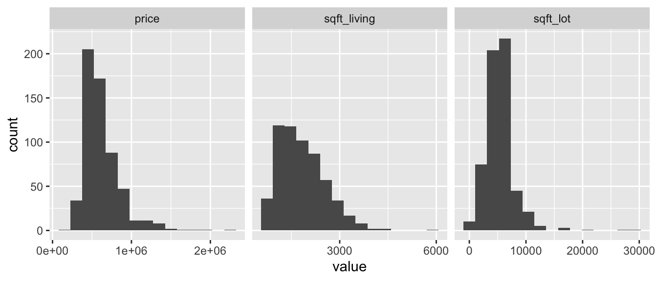
houses_98115 %>%
  tidyr::pivot_longer(cols = c(price, sqft_living, sqft_lot)) %>%
  ggplot(aes(value)) +
  geom_histogram(bins = 15) +
  facet_wrap(~name, scales = "free_x")

Now let’s make two scatterplots.

ggplot(houses_98115, aes(x = sqft_lot, y = price)) +
  geom_point()
ggplot(houses_98115, aes(x = sqft_living, y = price)) +
  geom_point()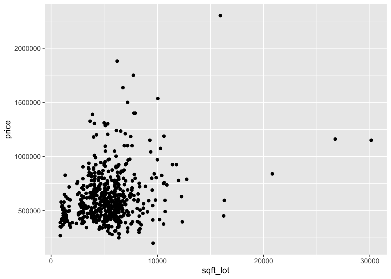

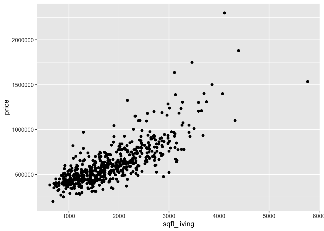
Looking at the two plots separately, it appears that the variance of price is not constant across the explanatory variables. Combining this with the fact that the variables are skewed, we take logs of all three variables:

log_houses <- fosdata::houses %>%
  filter(zipcode == "98115") %>%
  mutate(
    log_price = log(price),
    log_sqft_living = log(sqft_living),
    log_sqft_lot = log(sqft_lot)
  ) %>%
  select(matches("^log"))

The scatterplots are improved, though log of price versus log of lot size does not look great.

ggplot(log_houses, aes(x = log_sqft_lot, y = log_price)) +
  geom_point()
ggplot(log_houses, aes(x = log_sqft_living, y = log_price)) +
  geom_point()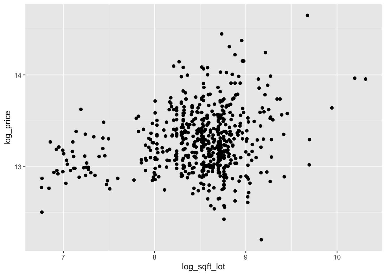

We continue by modeling the log of price on the log of the two explanatory variables. With only two explanatory variables, it is still possible to visualize the relationship. For scatterplots in three dimensions, we recommend plotly. We will not be utilizing all of the features of plotly, so we present the code that produces Figure 13.1 without fully explaining the syntax.

plotly::plot_ly(log_houses,
  x = ~log_sqft_living,
  y = ~log_sqft_lot,
  z = ~log_price,
  type = "scatter3d",
  marker = list(size = 2)
)

Figure 13.1: Three-dimensional plot created with plotly.

Plots made with plotly are interactive, so we recommend running the code yourself so that you can rotate and view the scatterplot. With a full view of the data, it seems reasonable that a plane could model the relationship between \(x\), \(y\), and \(z\). How would we find the equation of the plane that is the best fit? We write the equation of the plane as \(z = b_0 + b_1 x + b_2 y\) for some choices of \(b_0, b_1\), and \(b_2\). For each \(b_0, b_1\), and \(b_2\) we can predict the values of \(z\) at the values of the explanatory variables by computing \(\hat z_i = b_0 + b_1 x_i + b_2 y_i\). The associated error is \(\hat z_i - z_i\), and we find the values of \(b_0, b_1\), and \(b_2\) that minimize the sum of squares of the error. We denote the values that minimize the SSE as \(\hat \beta_0\), \(\hat \beta_1\), and \(\hat \beta_2\).

Model: Our model is \[ z_i = \beta_0 + \beta_1 x_i + \beta_2 y_i + \epsilon_i \] where \(\beta_0, \beta_1\), and \(\beta_2\) are unknown parameters, and \(\epsilon_i\) are independent, identically distributed normal random variables. The \(i\)th response is given by \(z_i\), and the \(i\)th predictors are \(x_i\) and \(y_i\).

For example, if \(b_0 = b_1 = b_2 = 1\), then we can compute the sum of squared error via

b_0 <- 1
b_1 <- 1
b_2 <- 1
log_houses %>%
  mutate(
    z_hat = b_0 + b_1 * log_sqft_living + b_2 * log_sqft_lot,
    resid = log_price - z_hat
  ) %>%
  summarize(SSE = sum(resid^2))

##       SSE
## 1 7961.38

Tryit 13.1

By hand, adjust the values of \(b_0, b_1\), and \(b_2\) in the code above to try and minimize the SSE.

We can find the values of \(b_0, b_1\), and \(b_2\) that minimize the SSE using lm. The format is very similar to the single explanatory variable case.

price_mod <- lm(log_price ~ log_sqft_living + log_sqft_lot,
  data = log_houses
)
summary(price_mod)

## 
## Call:
## lm(formula = log_price ~ log_sqft_living + log_sqft_lot, data = log_houses)
## 
## Residuals:
##      Min       1Q   Median       3Q      Max 
## -0.62790 -0.12085 -0.00189  0.12904  0.75567 
## 
## Coefficients:
##                 Estimate Std. Error t value Pr(>|t|)    
## (Intercept)      8.14199    0.19922   40.87   <2e-16 ***
## log_sqft_living  0.65130    0.02303   28.29   <2e-16 ***
## log_sqft_lot     0.03422    0.01755    1.95   0.0517 .  
## ---
## Signif. codes:  0 '***' 0.001 '**' 0.01 '*' 0.05 '.' 0.1 ' ' 1
## 
## Residual standard error: 0.211 on 580 degrees of freedom
## Multiple R-squared:  0.6021, Adjusted R-squared:  0.6007 
## F-statistic: 438.8 on 2 and 580 DF,  p-value: < 2.2e-16

We ignore most of the output for now and focus on the estimates of the coefficients. Namely, \(\hat \beta_0 = 8.14199\), \(\hat \beta_1 = 0.65130\), and \(\hat \beta_2 = 0.03422\).

For comparison, these coefficients lead to a SSE of 25.8:

beta_0 <- 8.14199
beta_1 <- 0.65130
beta_2 <- 0.03422
log_houses %>%
  mutate(
    z_hat = beta_0 + beta_1 * log_sqft_living + beta_2 * log_sqft_lot,
    resid = log_price - z_hat
  ) %>%
  summarize(SSE = sum(resid^2))

##       SSE
## 1 25.8307

This value is much smaller than the SSE we got from our first guess of \(b_0 = b_1 = b_2 = 1\)!

Tryit 13.2

Compute the SSE with \(b_0 = 8.15, b_1 = 0.65\), and \(b_2 = 0.034\) and confirm that the SSE increases.

Let’s use plotly to visualize the regression plane. We include the code for completeness, but do not explain the details of how to do this. Plotly produces interactive plots that do not render well on paper, so we recommend running this code in R to see the results.

# Compute a grid of x,y values for the plane
x <- seq(min(log_houses$log_sqft_living),
  max(log_houses$log_sqft_living),
  length.out = 10
)
y <- seq(min(log_houses$log_sqft_lot),
  max(log_houses$log_sqft_lot),
  length.out = 10
)
grid <- expand.grid(x, y) %>%
  rename(log_sqft_living = Var1, log_sqft_lot = Var2) %>%
  select(matches("^log")) %>%
  modelr::add_predictions(price_mod)
z <- reshape2::acast(grid, log_sqft_lot ~ log_sqft_living,
  value.var = "pred"
)

plotly::plot_ly(
  data = log_houses,
  x = ~log_sqft_living,
  y = ~log_sqft_lot,
  z = ~log_price,
  type = "scatter3d",
  marker = list(size = 2, color = "black")
) %>%
  plotly::add_trace(
    x = ~x,
    y = ~y,
    z = ~z,
    type = "surface"
  )

Let’s now examine the summary of lm when there are two explanatory variables.

summary(price_mod)

## 
## Call:
## lm(formula = log_price ~ log_sqft_living + log_sqft_lot, data = log_houses)
## 
## Residuals:
##      Min       1Q   Median       3Q      Max 
## -0.62790 -0.12085 -0.00189  0.12904  0.75567 
## 
## Coefficients:
##                 Estimate Std. Error t value Pr(>|t|)    
## (Intercept)      8.14199    0.19922   40.87   <2e-16 ***
## log_sqft_living  0.65130    0.02303   28.29   <2e-16 ***
## log_sqft_lot     0.03422    0.01755    1.95   0.0517 .  
## ---
## Signif. codes:  0 '***' 0.001 '**' 0.01 '*' 0.05 '.' 0.1 ' ' 1
## 
## Residual standard error: 0.211 on 580 degrees of freedom
## Multiple R-squared:  0.6021, Adjusted R-squared:  0.6007 
## F-statistic: 438.8 on 2 and 580 DF,  p-value: < 2.2e-16

We proceed through the summary line-by-line to explain what each value represents.

Call

This gives the call to lm that was used to create the model, in this case

lm(formula = log_price ~ log_sqft_living + log_sqft_lot, data = log_houses)

Having the call reproduced can be useful when you are comparing multiple models, or when a function creates a model for you without your typing it in directly.

Residuals

This gives the values of the estimated value of the response minus the actual value of the response. Our assumption is that \(Z = \beta_0 + \beta_1 X + \beta_2 Y + \epsilon\), where \(\epsilon\) is normal. In this case, we should expect that the residuals are symmetric about 0, so we would like to see that the median is approximately 0, the 1st and 3rd quartiles are about equal in absolute value, and the min and max are about equal in absolute value.

Coefficients

This gives the estimate for the coefficients, together with the standard error, \(t\)-value for use in a \(t\)-test of significance, and \(p\)-value. The \(p\)-value in row \(i\) is for the test of \(H_0: \beta_i = 0\) versus \(H_a: \beta_i \not= 0\). In this instance, we reject the null hypotheses that the slope associated with log_sqft_living is zero at the \(\alpha = .05\) level, and fail to reject that the slope of log_sqft_lot is zero at the \(\alpha = .05\) level. The \(\epsilon_i\) must be normal in order for these \(p\)-values to be accurate.

Residual standard error

This can be computed from the residuals as follows:

N <- nrow(log_houses)
sqrt(sum(residuals(price_mod)^2) / (N - 3))

## [1] 0.2110348

Recall our rule of thumb that we divide by the sample size minus the number of estimated parameters when estimating \(\sigma\). In this case, there are three estimated parameters. The degrees of freedom is just the number of samples minus the number of parameters estimated.

Multiple R-squared

This can be interpreted as the percent of variance in the response that is explained by the model. It can be computed as follows:

var_response <- var(log_houses$log_price)
var_residuals <- var(residuals(price_mod))
(var_response - var_residuals) / var_response

## [1] 0.6020751

The Adjusted \(R^2\) uses the residual standard error (that has been adjusted for the number of parameters) rather than the raw variance of the residuals.

(var_response - sum(residuals(price_mod)^2) / (N - 3)) / (var_response)

## [1] 0.600703

The multiple \(R^2\) value will increase with the addition of more variables, where the adjusted \(R^2\) has a penalty for adding variables, so can either increase or decrease when a new variable is added.

F statistic

The test statistic which is used to test \(H_0: \beta_1 = \beta_2 = \cdots = 0\) versus not all of the slopes are 0. Note this does not include a test for the intercept. The \(\epsilon_i\) must be normal for this to be accurate. We compute the value via

ssresid <- sum(residuals(price_mod)^2)
ssresponse <- sum((log_houses$log_price - mean(log_houses$log_price))^2)
(ssresponse - ssresid) / 2 / (ssresid / (N - 3))

## [1] 438.7808

13.2 Categorical variables

This section details how R incorporates categorical variables into linear models, expanding on the brief discussion in Section 12.1.1. Let’s expand the ZIP codes in our model to include a ZIP code in the suburbs, which may have different characteristics. These are the same ZIP codes we used for data visualization in Section 7.3.1.

houses_2zips <- filter(fosdata::houses, zipcode %in% c("98038", "98115"))

We again take the log of price, sqft_lot and sqft_living.

houses_2zips <- mutate(houses_2zips,
  log_sqft_lot = log(sqft_lot),
  log_sqft_living = log(sqft_living),
  log_price = log(price)
)
houses_2zips$zipcode <- factor(houses_2zips$zipcode)

Alert 13.1

It would be a mistake to treat zipcode as a numeric variable! It is converted to a factor instead.

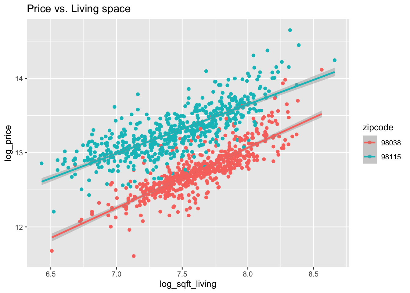
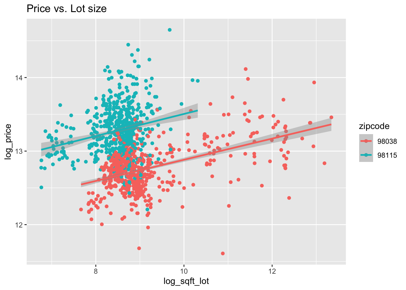
Figure 13.2: House price as a function of living space and lot size in two Seattle area ZIP codes (all variables logged).

Figure 13.2 shows the dependence of price on living space, lot size, and zip code.

13.2.1 Equal slopes model

From Figure 13.2, it appears that 98038 and 98115 may have similar slopes for log_price when modeled by log_sqft_living and log_sqft_lot, although changing ZIP code causes a vertical shift. Based on that, it is reasonable to model the price by two parallel planes, one for each ZIP code. To do this with lm, we include all three explanatory variables on the right-hand side of the formula.

house_modE <- lm(log_price ~ log_sqft_living + log_sqft_lot + zipcode,
  data = houses_2zips
)
summary(house_modE)

## 
## Call:
## lm(formula = log_price ~ log_sqft_living + log_sqft_lot + zipcode, 
##     data = houses_2zips)
## 
## Residuals:
##      Min       1Q   Median       3Q      Max 
## -0.96278 -0.09510  0.00084  0.09298  0.68666 
## 
## Coefficients:
##                 Estimate Std. Error t value Pr(>|t|)    
## (Intercept)      6.82806    0.12150   56.20   <2e-16 ***
## log_sqft_living  0.67827    0.01562   43.43   <2e-16 ***
## log_sqft_lot     0.08329    0.00659   12.64   <2e-16 ***
## zipcode98115     0.69684    0.01182   58.97   <2e-16 ***
## ---
## Signif. codes:  0 '***' 0.001 '**' 0.01 '*' 0.05 '.' 0.1 ' ' 1
## 
## Residual standard error: 0.1857 on 1169 degrees of freedom
## Multiple R-squared:  0.7999, Adjusted R-squared:  0.7994 
## F-statistic:  1558 on 3 and 1169 DF,  p-value: < 2.2e-16

The equation to predict the log of price comes from the coefficients of the model: \[ \widehat{\log(\text{price})} = 6.83 + 0.678\cdot \log(\text{sqft\_living}) + 0.083\cdot \log(\text{sqft\_lot}) + 0.697\cdot\text{zipcode98115}. \]

The zipcode98115 variable is a dummy variable that takes two values. It is 1 when the ZIP code is 98115 and otherwise 0. Both ZIP codes have the same coefficients on the living and lot variables, but there is an additive adjustment when the house is in ZIP code 98115 rather than in 98038. This number, 0.697, could be interpreted as the amount that \(\log(\text{price})\) increases between ZIP code 98038 and 98115. Exponentiation turns this additive factor into a multiplicative factor. Since \(e^{0.697} \approx 2\), properties in 98115 are worth about twice as much as comparably sized properties in 98038.

The ZIP code 98038 is the “base” level of the zipcode variable. The base level is whichever level appears first when listing the levels of a factor, for example with levels(houses_2zips$zipcode). If you want to change the base level to 98115, reorder the factor levels so 98115 comes first:

houses_2zips <- houses_2zips %>%
  mutate(zipcode = factor(zipcode, levels = c("98115", "98038")))
house_modE <- lm(log_price ~ log_sqft_living + log_sqft_lot + zipcode,
  data = houses_2zips
)
summary(house_modE)$coefficients

##                    Estimate Std. Error   t value      Pr(>|t|)
## (Intercept)      7.52489382 0.11779971  63.87871  0.000000e+00
## log_sqft_living  0.67827046 0.01561607  43.43414 3.778832e-246
## log_sqft_lot     0.08329213 0.00659035  12.63850  2.059559e-34
## zipcode98038    -0.69683562 0.01181683 -58.96974  0.000000e+00

13.2.2 Interaction terms

Although the slopes of the lines in Figure 13.2 appear similar, a more accurate model of house prices might include variable slopes for each ZIP code. Adding interaction terms to the model allows the coefficients to vary with ZIP code. Interaction terms involve two variables, separated by a colon (:) character. In the case of house prices, we add log_sqft_living:zipcode and log_sqft_lot:zipcode to the model.

house_modV <- lm(
  log_price ~ log_sqft_living + log_sqft_lot + zipcode +
    log_sqft_living:zipcode + log_sqft_lot:zipcode,
  data = houses_2zips
)
summary(house_modV)

## 
## Call:
## lm(formula = log_price ~ log_sqft_living + log_sqft_lot + zipcode + ...
## Residuals:
##      Min       1Q   Median       3Q      Max 
## -0.94919 -0.09573  0.00371  0.09358  0.75567 
## 
## Coefficients:
##                              Estimate Std. Error t value Pr(>|t|)    
## (Intercept)                   8.14199    0.17375  46.861  < 2e-16 ***
## log_sqft_living               0.65130    0.02008  32.433  < 2e-16 ***
## log_sqft_lot                  0.03422    0.01531   2.236 0.025558 *  
## zipcode98038                 -1.81575    0.25254  -7.190 1.16e-12 ***
## log_sqft_living:zipcode98038  0.08308    0.03175   2.617 0.008995 ** 
## log_sqft_lot:zipcode98038     0.05716    0.01695   3.373 0.000769 ***
## ---
## Signif. codes:  0 '***' 0.001 '**' 0.01 '*' 0.05 '.' 0.1 ' ' 1
## 
## Residual standard error: 0.184 on 1167 degrees of freedom
## Multiple R-squared:  0.8038, Adjusted R-squared:  0.8029 
## F-statistic:   956 on 5 and 1167 DF,  p-value: < 2.2e-16

From the summary¹¹³, we see that there is a small but statistically significant difference between the linear relationship of log of price to the other variables in the two ZIP codes.

To estimate the log price of a house in ZIP code 98115 (recall we changed the base level), use \[ \widehat{\log(\text{price})} = 8.142 + 0.651 \cdot \log(\text{sqft\_living}) + 0.034 \cdot \log(\text{sqft\_lot}). \] To estimate the expected value of the log of the price of a home in ZIP code 98038, we must adjust each coefficient by its interaction term. So \[ \widehat{\log(\text{price})} = 8.142 - 1.816 + (0.651 + 0.083)\cdot \log(\text{sqft\_living}) + (0.03422 + 0.05716) \cdot \log(\text{sqft\_lot}). \]

The predict function works on these models as well as on simple linear models. Let’s check our results using predict for a house in ZIP code 98038 with log_sqft_living = 8 and log_sqft_lot = 9.

predict(house_modV,
  newdata = data.frame(
    log_sqft_living = 8,
    log_sqft_lot = 9, zipcode = "98038"
  )
)

##        1 
## 13.02381

log_sqft_living <- 8
log_sqft_lot <- 9
8.14199 - 1.81575 + (0.65130 + 0.08308) * log_sqft_living +
  (0.03422 + 0.05716) * log_sqft_lot # agrees with above

## [1] 13.0237

Finally, we note that predict has options for prediction intervals and confidence intervals which work for multiple linear regression as well. If we want a 95% prediction interval for the log price of a house with log_sqft_living = 8 and log_sqft_lot = 9, we see that it is \([12.66, 13.39]\), which corresponds roughly to \([315000 ,651000]\) in the non-log scale.

predict(house_modV,
  newdata = data.frame(
    log_sqft_living = 8,
    log_sqft_lot = 9, zipcode = "98038"
  ),
  interval = "prediction"
) %>% exp()

##        fit      lwr      upr
## 1 453072.1 315496.9 650638.2

13.2.3 Cross validation

We have seen two models of housing price on living space, lot size, and ZIP code. One model assumed equal slopes, the other included interaction terms. This choice of models is another example of the bias-variance tradeoff introduced in Section 11.8. Interaction terms decrease the bias of the model (by fitting the data better) but come at a cost of additional variance. In this section we apply leave one out cross validation to compare the predictive value of an equal slopes model to a model including interaction terms in a new data set.

Example 13.1

The data set hot_dogs is in the fosdata package.

hot_dogs <- fosdata::hot_dogs

This data comes from Consumer Reports and describes the sodium and calorie content various brands of hot dogs. The categorical variable type is one of Beef, Meat, or Poultry.

Figure 13.3 shows sodium content as explained by calories and type of hot dog.

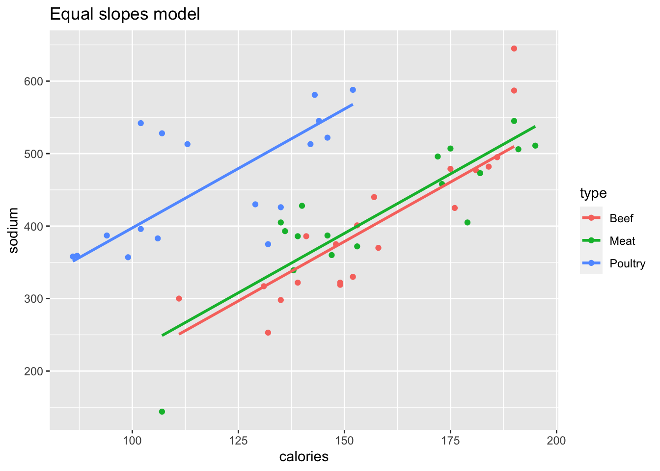
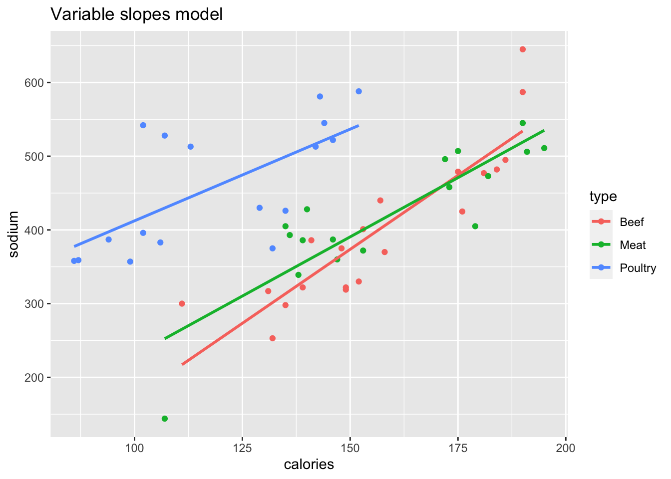
Figure 13.3: Two models of hot dog sodium content.

The left plot in Figure 13.3 is an equal slopes model, generated by

hd_Eslope <- lm(sodium ~ calories + type, data = hot_dogs)

The right plot shows a variable slopes model, which includes the interaction term calories:type. A shortcut to include all interaction terms is to use * rather than + between the explanatory variables:

hd_Vslope <- lm(sodium ~ calories * type, data = hot_dogs)
summary(hd_Vslope)

## 
## Call:
## lm(formula = sodium ~ calories * type, data = hot_dogs)
## 
## Residuals:
##      Min       1Q   Median       3Q      Max 
## -116.916  -28.180   -8.961   35.798  124.694 
## 
## Coefficients:
##                       Estimate Std. Error t value Pr(>|t|)    
## (Intercept)          -228.3313    87.5770  -2.607  0.01213 *  
## calories                4.0133     0.5529   7.259 2.96e-09 ***
## typeMeat              137.1460   123.3106   1.112  0.27159    
## typePoultry           391.9615   114.0463   3.437  0.00122 ** 
## calories:typeMeat      -0.8016     0.7733  -1.037  0.30511    
## calories:typePoultry   -1.5263     0.8195  -1.862  0.06868 .  
## ---
## Signif. codes:  0 '***' 0.001 '**' 0.01 '*' 0.05 '.' 0.1 ' ' 1
## 
## Residual standard error: 54.57 on 48 degrees of freedom
## Multiple R-squared:  0.7065, Adjusted R-squared:  0.6759 
## F-statistic: 23.11 on 5 and 48 DF,  p-value: 9.698e-12

Observe that the type variable has base level Beef, and that there is a 0/1 valued variable for each of the other two levels, Meat and Poultry. From the summary, we see that the interaction terms are not significant at the 0.05 level.

Now we perform LOOCV on the two models. For the equal slopes model:

loo_Eslope <- function(k) {
  train <- hot_dogs[-k, ]
  test <- hot_dogs[k, ]
  hd_Eslope <- lm(sodium ~ calories + type, data = train)
  test$sodium - predict(hd_Eslope, test)
}
errs_E <- sapply(1:nrow(hot_dogs), loo_Eslope)
mean(errs_E^2)

## [1] 3345.211

For the variable slopes model:

loo_Vslope <- function(k) {
  train <- hot_dogs[-k, ]
  test <- hot_dogs[k, ]
  hd_Vslope <- lm(sodium ~ calories * type, data = train)
  test$sodium - predict(hd_Vslope, test)
}
errs_V <- sapply(1:nrow(hot_dogs), loo_Vslope)
mean(errs_V^2)

## [1] 3562.832

For this data set, LOOCV prefers the equal slopes model, whose SSE is 3345, about 217 smaller than the SSE for the variable slopes model.

13.3 Variable selection

One of the goals of linear regression is to be able to choose a parsimonious set of explanatory variables: a small set of variables that have great explanatory power. The problem of choosing a parsimonious set is one of variable selection, and there are many ways to approach this problem.

This section presents one possible approach to variable selection, stepwise regression using \(p\)-values. The method proceeds as follows:

1. Organize the variables that naturally belong together into groups, if possible.
2. Remove the non-significant variables in a group in decreasing order of \(p\)-value. Check after each removal to see whether the significance of other variables has changed. Keep categorical variables if any of the levels of the variable are significant.
3. Once all remaining variables in the group are significant, use anova to test whether the collection of removed variables was significant. If so, test one-by-one to try to find one to put back in the model.
4. Move to the next group of variables and continue until all variables in the model are significant.

The rest of this section illustrates the process with an extended example.

The data set fosdata::conversation is adapted from a psychological study by Manson et. al.¹¹⁴ This study had 210 university students participate in a 10-minute conversation in small groups. After the conversation, the students were paired up to play a game known as the “prisoner’s dilemma.” The participants also provided various demographic information, and took a test to indicate whether they suffered from subclinical psychopathy. The goal of the study was to determine whether and/or how conversational behavior depends on demographic data.

To illustrate variable selection, we are going to model the proportion_words variable on the other variables in the data set. The proportion_words variable gives the proportion of words spoken by that student among all words spoken by everyone during the conversation.

Tryit 13.3

Read the help page for conversation. Use the summary command to get an overview of all variables in the data set at once. Observe that most of the numeric variables have been standardized so as to have approximately mean 0 and standard deviation 1.

Many of the variables in this data refer to the prisoner’s dilemma portion of the experiment. That part of the experiment happened after the conversations, so we will omit them from our model. Those variables include camera and eight more that all begin with the string indiv. The variable oldest has 72 missing values and is poorly documented, so we remove it as well. Also as part of this data cleanup, we convert gender to a factor.

converse <- fosdata::conversation %>%
  select(!camera) %>%
  select(!matches("^indiv")) %>%
  select(!oldest) %>%
  mutate(gender = factor(gender, levels = c(0, 1), labels = c("M", "F")))

This leaves 18 variables, consisting of 17 explanatory variables and our one response variable proportion_words. These 17 explanatory variables split naturally into two groups: demographic data and conversational data. The demographic data includes data on gender, appearance, psychopathy, the student’s major, fighting ability (as estimated based on a picture), and more. The conversational data measures the number of interruptions, the number of times that a person started a new topic on a per word basis, and the proportion of times a person started a new topic.

Let’s explore with some visualizations. We arbitrarily pick two of the explanatory variables to plot versus the response:

ggplot(converse, aes(x = f1_psychopathy, y = proportion_words)) +
  geom_point() +
  geom_smooth(method = "lm")
ggplot(converse, aes(x = interruptions_per_min, y = proportion_words)) +
  geom_point() +
  geom_smooth(method = "lm")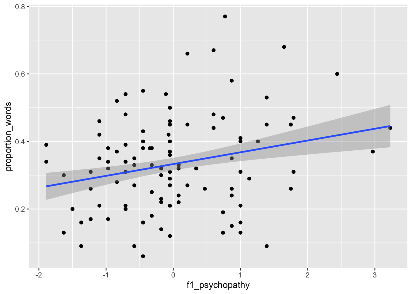

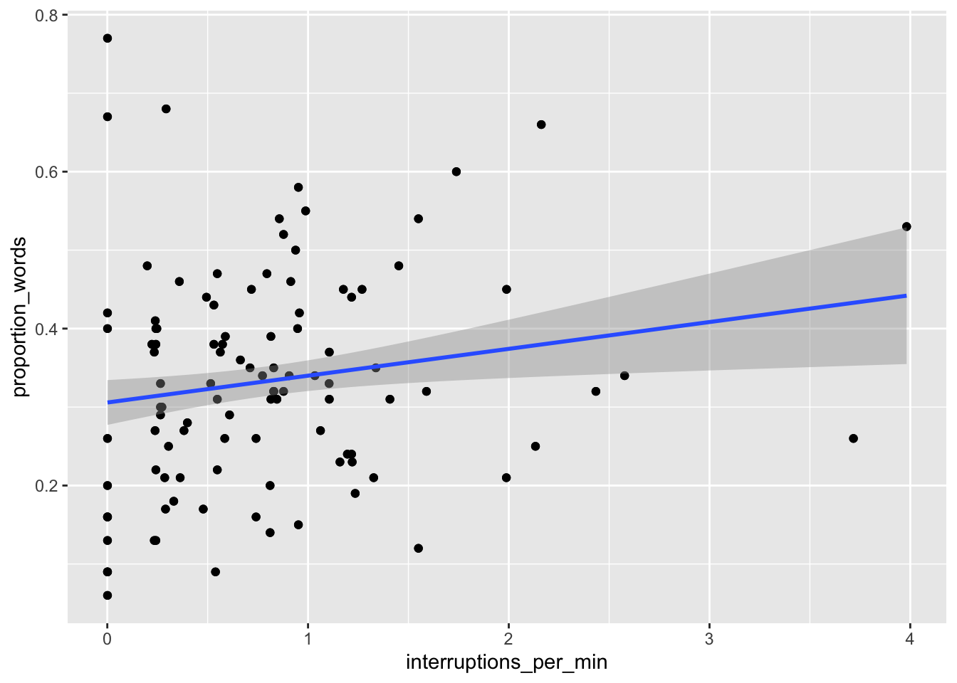
Figure 13.4: Proportion of words spoken modeled on psychopathy (left) and interruptions per minute (right).

The results, in Figure 13.4, suggest that neither of the two variables have strong predictive ability for the response by themselves. Perhaps with all of the variables, things will look better:

mod <- lm(proportion_words ~ ., data = converse)
summary(mod)

## 
## Call:
## lm(formula = proportion_words ~ ., data = converse)
## 
## Residuals:
##       Min        1Q    Median        3Q       Max 
## -0.183163 -0.040952  0.002491  0.044088  0.188120 
## 
## Coefficients:
##                          Estimate Std. Error t value Pr(>|t|)    
## (Intercept)             0.2959771  0.0305151   9.699  < 2e-16 ***
## genderF                 0.0051863  0.0118649   0.437  0.66252    
## f1_psychopathy         -0.1579680  0.4577533  -0.345  0.73040    
## f2_psychopathy         -0.0980854  0.2457922  -0.399  0.69029    
## total_psychopathy       0.2237067  0.5963622   0.375  0.70799    
## attractiveness         -0.0022099  0.0055057  -0.401  0.68859    
## fighting_ability       -0.0286368  0.0086793  -3.299  0.00115 ** 
## strength                0.0186639  0.0085663   2.179  0.03057 *  
## height                 -0.0057262  0.0055482  -1.032  0.30333    
## median_income           0.0001271  0.0002090   0.608  0.54379    
## highest_class_rank      0.0242887  0.0115059   2.111  0.03607 *  
## major_presige          -0.0005630  0.0005683  -0.991  0.32313    
## dyad_status_difference -0.0178477  0.0070620  -2.527  0.01230 *  
## proportion_seque...rts  0.4855446  0.0409178  11.866  < 2e-16 ***
## interruptions_per_min   0.1076160  0.0144719   7.436 3.35e-12 ***
## sequence_starts_...100 -0.0493571  0.0061830  -7.983 1.28e-13 ***
## interruptions_pe...100 -0.0708835  0.0094431  -7.506 2.22e-12 ***
## affect_words           -0.0039201  0.0027227  -1.440  0.15155    
## ---
## Signif. codes:  0 '***' 0.001 '**' 0.01 '*' 0.05 '.' 0.1 ' ' 1
## 
## Residual standard error: 0.07303 on 192 degrees of freedom
## Multiple R-squared:  0.751,  Adjusted R-squared:  0.729 
## F-statistic: 34.07 on 17 and 192 DF,  p-value: < 2.2e-16

A couple of things to notice. First, two of the other three conversation variables are significant when predicting the proportion of words spoken. Second, the multiple \(R^2\) is .751, which means that about 75% of the variance in the proportion of words spoken is explained by the explanatory variables.

Let’s start removing variables in groups. The three psychopathy variables have high \(p\)-values, so we begin with them, removing one at a time.

To remove variables from an existing model, use the update command. The update command takes the model as its first argument and the update we are making as its second. The second argument is given as a formula ~ . - variable_name, which means we update by subtracting the named variable.

Rather than show the full model at each step, we show only selected variables and format them nicely (using kable).

mod2 <- update(mod, ~ . - f1_psychopathy)

term	estimate	std.error	statistic	p.value
(Intercept)	0.295	0.030	9.745	0.000
f2_psychopathy	-0.013	0.008	-1.656	0.099
total_psychopathy	0.018	0.009	2.102	0.037

summary(mod2)$r.squared

## [1] 0.7508613

summary(mod2)$adj.r.squared

## [1] 0.7302073

We see that after removing f1_psychopathy, the variables total_psychopathy and f2_psychopathy had much smaller \(p\)-values than before. It is common to see such large changes in significance when removing variables that are linked or correlated in some way. Also, note that the \(R^2\) did not decrease much when we removed f1_psychopathy, and the adjusted \(R^2\) increased from .729 to .730. These are good signs that it is OK to remove f1_psychopathy.

In the updated model, total_psychopathy has coefficient significantly different from 0 (\(p = .037\)), while f2_psychopathy is not significant at the \(\alpha = .05\) level. Since f2_psychopathy is weaker, we try removing it too:

mod3 <- update(mod2, ~ . - f2_psychopathy)

term	estimate	std.error	statistic	p.value
(Intercept)	0.296	0.030	9.731	0.000
total_psychopathy	0.007	0.006	1.293	0.198

summary(mod3)$r.squared

## [1] 0.7473232

summary(mod3)$adj.r.squared

## [1] 0.7277863

Here we get conflicting information about whether to remove f2_psychopathy. The variable was not significant at the \(\alpha = .05\) level, but the adjusted \(R^2\) decreased from .730 to .728 when we removed it.

Different variable selection techniques would make different choices at this point. The \(p\)-value technique determines that total_psychopathy is not significant (\(p = 0.198\)) so it should be removed.

mod4 <- update(mod3, ~ . - total_psychopathy)

Here is the full model summary after removing all three psychopathy variables.

summary(mod4)

## 
## Call:
## lm(formula = proportion_words ~ gender + attractiveness + fighting_a...
## Residuals:
##       Min        1Q    Median        3Q       Max 
## -0.180736 -0.038420 -0.000994  0.043020  0.202987 
## 
## Coefficients:
##                          Estimate Std. Error t value Pr(>|t|)    
## (Intercept)             0.2933090  0.0303800   9.655  < 2e-16 ***
## genderF                -0.0037965  0.0108581  -0.350 0.726983    
## attractiveness         -0.0028329  0.0055096  -0.514 0.607706    
## fighting_ability       -0.0304228  0.0083761  -3.632 0.000359 ***
## strength                0.0211761  0.0083132   2.547 0.011628 *  
## height                 -0.0082203  0.0053578  -1.534 0.126585    
## median_income           0.0001295  0.0002088   0.620 0.535722    
## highest_class_rank      0.0244283  0.0114397   2.135 0.033976 *  
## major_presige          -0.0004255  0.0005441  -0.782 0.435162    
## dyad_status_difference -0.0153037  0.0069836  -2.191 0.029610 *  
## proportion_seque...rts  0.5013595  0.0399347  12.554  < 2e-16 ***
## interruptions_per_min   0.1138530  0.0141768   8.031 8.97e-14 ***
## sequence_starts_...100 -0.0481660  0.0061777  -7.797 3.73e-13 ***
## interruptions_pe...100 -0.0731355  0.0093695  -7.806 3.53e-13 ***
## affect_words           -0.0050216  0.0026643  -1.885 0.060946 .  
## ---
## Signif. codes:  0 '***' 0.001 '**' 0.01 '*' 0.05 '.' 0.1 ' ' 1
## 
## Residual standard error: 0.07331 on 195 degrees of freedom
## Multiple R-squared:  0.7451, Adjusted R-squared:  0.7268 
## F-statistic: 40.72 on 14 and 195 DF,  p-value: < 2.2e-16

The adjusted \(R^2\) fell again, this time to .727. Now that we have removed all of the variables related to psychopathy, we can check to see whether as a group they are significant. That is, we will test \(H_0\) (the coefficients of the psychopathy variables are all 0) versus \(H_a\) (not all of the coefficients are zero).

anova(mod4, mod)

## Analysis of Variance Table
## 
## Model 1: proportion_words ~ gender + attractiveness + fighting_ability...
## Model 2: proportion_words ~ gender + f1_psychopathy + f2_psychopathy +...
##   Res.Df    RSS Df Sum of Sq      F Pr(>F)
## 1    195 1.0481                           
## 2    192 1.0240  3  0.024138 1.5087 0.2136

With a \(p\)-value of .2136, we do not reject the null hypothesis that all of the coefficients are zero, and so we leave the psychopathy variables out of the model. If we had rejected the null hypothesis, then we would have needed to add back in one or more of the variables to the model. It is important when doing stepwise variable selection that you periodically check to see whether you need to add back in one or more of the variables that you removed.

Next, we begin removing variables that describe the person, such as gender and attractiveness. We step in order of decreasing \(p\)-values within that group of variables.

mod5 <- update(mod4, ~ . - gender)
mod6 <- update(mod5, ~ . - attractiveness)
mod7 <- update(mod6, ~ . - median_income)
summary(mod7)

## 
## Call:
## lm(formula = proportion_words ~ fighting_ability + strength +   ...
## Residuals:
##       Min        1Q    Median        3Q       Max 
## -0.181215 -0.037676 -0.000914  0.042230  0.202280 
## 
## Coefficients:
##                          Estimate Std. Error t value Pr(>|t|)    
## (Intercept)             0.3024526  0.0214860  14.077  < 2e-16 ***
## fighting_ability       -0.0300948  0.0082729  -3.638 0.000351 ***
## strength                0.0207458  0.0082203   2.524 0.012397 *  
## height                 -0.0080111  0.0052692  -1.520 0.130012    
## highest_class_rank      0.0243218  0.0112871   2.155 0.032382 *  
## major_presige          -0.0004917  0.0005239  -0.939 0.349084    
## dyad_status_difference -0.0144526  0.0067093  -2.154 0.032439 *  
## proportion_seque...rts  0.5008202  0.0393863  12.716  < 2e-16 ***
## interruptions_per_min   0.1127051  0.0138752   8.123 4.81e-14 ***
## sequence_starts_...100 -0.0488678  0.0060006  -8.144 4.22e-14 ***
## interruptions_pe...100 -0.0725000  0.0092657  -7.825 2.99e-13 ***
## affect_words           -0.0048069  0.0025190  -1.908 0.057807 .  
## ---
## Signif. codes:  0 '***' 0.001 '**' 0.01 '*' 0.05 '.' 0.1 ' ' 1
## 
## Residual standard error: 0.07289 on 198 degrees of freedom
## Multiple R-squared:  0.7442, Adjusted R-squared:   0.73 
## F-statistic: 52.37 on 11 and 198 DF,  p-value: < 2.2e-16

anova(mod7, mod4)

## Analysis of Variance Table
## 
## Model 1: proportion_words ~ fighting_ability + strength + height + hig...
## Model 2: proportion_words ~ gender + attractiveness + fighting_ability...
##   Res.Df    RSS Df Sum of Sq      F Pr(>F)
## 1    198 1.0520                           
## 2    195 1.0481  3 0.0038477 0.2386 0.8693

After removing those three variables, the adjusted \(R^2\) is back up to 0.73, and ANOVA indicates it is not necessary to put any of the variables back in. We continue.

mod8 <- update(mod7, ~ . - major_presige)
mod9 <- update(mod8, ~ . - height)
mod10 <- update(mod9, ~ . - dyad_status_difference)
anova(mod10, mod7)

## Analysis of Variance Table
## 
## Model 1: proportion_words ~ fighting_ability + strength + highest_clas...
## Model 2: proportion_words ~ fighting_ability + strength + height + hig...
##   Res.Df    RSS Df Sum of Sq      F  Pr(>F)  
## 1    201 1.0893                              
## 2    198 1.0520  3  0.037357 2.3438 0.07427 .
## ---
## Signif. codes:  0 '***' 0.001 '**' 0.01 '*' 0.05 '.' 0.1 ' ' 1

summary(mod10)

## 
## Call:
## lm(formula = proportion_words ~ fighting_ability + strength +   ...
## Residuals:
##       Min        1Q    Median        3Q       Max 
## -0.192950 -0.041033  0.003062  0.042783  0.211376 
## 
## Coefficients:
##                         Estimate Std. Error t value Pr(>|t|)    
## (Intercept)             0.295980   0.020301  14.580  < 2e-16 ***
## fighting_ability       -0.033053   0.008021  -4.121 5.52e-05 ***
## strength                0.021673   0.008193   2.645  0.00881 ** 
## highest_class_rank      0.023024   0.011185   2.058  0.04084 *  
## proportion_seque...rts  0.502863   0.039371  12.772  < 2e-16 ***
## interruptions_per_min   0.113354   0.013994   8.100 5.22e-14 ***
## sequence_starts_...100 -0.048002   0.005906  -8.128 4.41e-14 ***
## interruptions_pe...100 -0.072946   0.009305  -7.840 2.59e-13 ***
## affect_words           -0.005876   0.002418  -2.430  0.01597 *  
## ---
## Signif. codes:  0 '***' 0.001 '**' 0.01 '*' 0.05 '.' 0.1 ' ' 1
## 
## Residual standard error: 0.07362 on 201 degrees of freedom
## Multiple R-squared:  0.7351, Adjusted R-squared:  0.7246 
## F-statistic: 69.73 on 8 and 201 DF,  p-value: < 2.2e-16

The adjusted \(R^2\) has fallen back down to .7246, but that is not a big price to pay for removing so many variables from the model. ANOVA does not reject \(H_0\) that all the coefficients of the variables that we removed are zero at the \(\alpha = .05\) level. We are left with 8 significant explanatory variables.

Let’s check the diagnostic plots.

plot(mod10)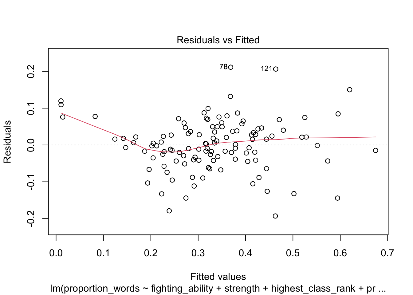

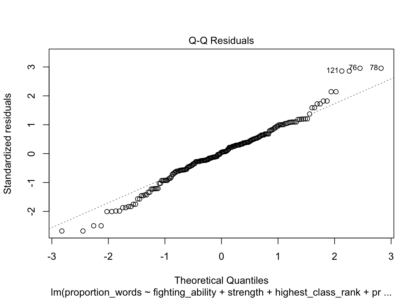
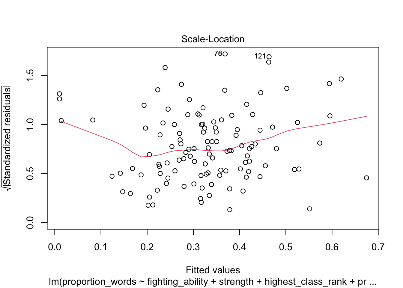
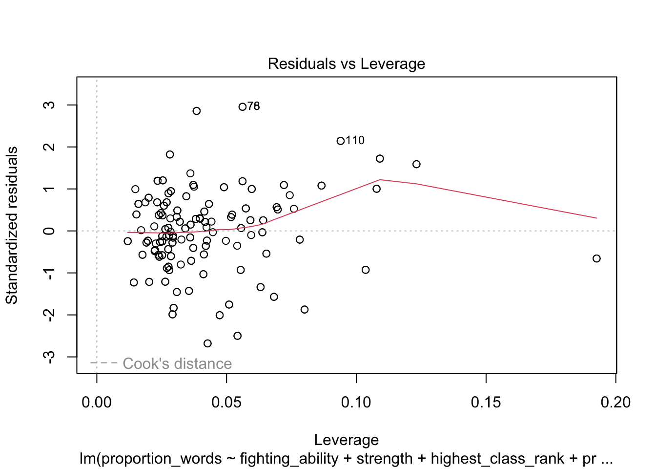
These look pretty good, except that there may be 3-4 values that don’t seem to be following the rest of the trend. See for example the residuals versus fitted plot with the 4 values on the left.

Doing stepwise regression like this is not without its detractors. One issue is that the final model is very much dependent on the order in which we proceed. If we had removed f2_psychopathy first, how would that have affected things? Can we justify our decision to remove f1_psychopathy first? Certainly not. The resulting model that we obtained is simply a model for the response, not necessarily the best one. It is also very possible that the variables that we removed are also good predictors of the response. We should not make the conclusion that the other variables aren’t related.

That being said, stepwise regression for variable selection is quite common in practice, which is why we include it in this book.

The technique we used above was based on \(p\)-values. One can also use other measures of goodness of fit of a model to perform stepwise regression. A common one is the Akaike Information Criterion (AIC). The AIC algorithm is nice because at each decision point, it tests what would happen if we add back in any of the variables that we have removed, as well as what would happen if we remove any of the variables that we currently have. We won’t explain how AIC works, but we show how to use an implementation of it from the MASS package to find a parsimonious model

mod_aic <- MASS::stepAIC(mod, trace = FALSE)
summary(mod_aic)

## 
## Call:
## lm(formula = proportion_words ~ f2_psychopathy + total_psychopathy +...
## Residuals:
##       Min        1Q    Median        3Q       Max 
## -0.189974 -0.036895  0.000572  0.044182  0.190963 
## 
## Coefficients:
##                         Estimate Std. Error t value Pr(>|t|)    
## (Intercept)             0.304026   0.020184  15.063  < 2e-16 ***
## f2_psychopathy         -0.013849   0.007641  -1.812 0.071434 .  
## total_psychopathy       0.018827   0.007876   2.390 0.017773 *  
## fighting_ability       -0.032058   0.008090  -3.963 0.000103 ***
## strength                0.020196   0.008139   2.481 0.013919 *  
## highest_class_rank      0.024566   0.011126   2.208 0.028394 *  
## dyad_status_difference -0.015754   0.006712  -2.347 0.019909 *  
## proportion_seque...rts  0.479287   0.039657  12.086  < 2e-16 ***
## interruptions_per_min   0.106362   0.014115   7.536 1.70e-12 ***
## sequence_starts_...100 -0.047826   0.005855  -8.168 3.63e-14 ***
## interruptions_pe...100 -0.071390   0.009274  -7.698 6.42e-13 ***
## affect_words           -0.005436   0.002393  -2.272 0.024170 *  
## ---
## Signif. codes:  0 '***' 0.001 '**' 0.01 '*' 0.05 '.' 0.1 ' ' 1
## 
## Residual standard error: 0.07246 on 198 degrees of freedom
## Multiple R-squared:  0.7472, Adjusted R-squared:  0.7332 
## F-statistic: 53.21 on 11 and 198 DF,  p-value: < 2.2e-16

In this case, the AIC derived model includes all of the variables that we included, plus f2_psychopathy, total_psychopathy, and dyad_status_difference. These variables do not all pass the \(p\)-value test, but notice that the adjusted \(R^2\) of the AIC derived model is higher than the adjusted \(R^2\) of the model that we chose using \(p\)-values. The two models have their pros and cons, and as is often the case, there is not just one final model that could make sense.

Vignette: External data formats

By this point in the book, we hope that you are comfortable doing many tasks in R. We like to imagine that when someone gives you data in the future, your first thought will be to open it up in R. Unfortunately, not everyone is as civilized as we are, and they may have saved their data in a format that doesn’t interact well with R. This vignette gives some guidance for what to do in that case.

As a general recommendation, never make modifications directly to the original data. That data should stay in the exact same state, and ideally, you would document every change and decision that you make while getting the data ready to be read into R. In particular, never write over the original data set.

Text formats

Text data is data stored as a sequence of simple characters (ASCII or Unicode, usually). It is easy to inspect and manipulate with any text editor. On the other hand, it typically does not include formatting or metadata (information about the data), and may be larger in size than some compressed formats. Despite, or really because of, their simplicity, textual data formats have proven to be the best storage format for interoperability and resistance to loss over time. If you have important data to release to the world, do the world a favor and make it available in a text format.

The most popular textual format is “comma separated values”, or CSV. CSV files have the .csv extension, and can be read and written with read.csv and write.csv:

# make some data
mydata <- data.frame(
  number = 1:10,
  letter = sample(c("A", "B", "C", "D"), 10, replace = TRUE)
)
# write it to a CSV
write.csv(mydata, file = "myfile.csv")
# read it back
mydata <- read.csv("myfile.csv")

Within a CSV file, each record is a row, and within that row data is separated into fields. The first row of a CSV file should contain the names of the fields, or variables. If it doesn’t, specify that header = FALSE and R will assign generic variable names to your columns.

The default field separator is a comma, hence the C in CSV. You may specify a different separator to read.csv. For example, files with the .tsv extension are tab separated and need the sep = "\t" option.

Other text formats with records in rows and variables in columns can be read with read.table, and in fact read.csv is just a wrapper that eventually calls read.table. Another possible approach for reading text files is with scan, which reads typed data. The readr package, part of the tidyverse, is also a powerful tool.

JSON is a text based format that is growing in popularity. Unlike row and column formatted table data, JSON is hierarchical, allowing for complicated object structures and relationships. Since R works most naturally with rectangular data, dealing with JSON is inherently challenging. R does provide packages (rjson, jsonlite) that will read JSON formats, but some data manipulation will almost certainly be required after loading.

Spreadsheets

Excel spreadsheet data is stored in files with .xls or .xlsx extensions. The readxl package provides readxl::read_xls("your_file_name.xls", sheet = 1) or readxl::read_xlsx(your_file_name.xlsx, sheet = 1) to import Excel data. Unfortunately, the readxl commands will only work well if the file was created by someone who understands the importance of rectangular data. Many, if not most, of the data that is stored in Excel format has data and metadata stored in the file itself. For example, cells might be merged for formatting, there may be 5 rows of headers describing the variables, or there might be cells performing computations – those aren’t data!

Working with complex Excel spreadsheets inside of R is possible, but quite challenging. It is almost always easier to open the file in a spreadsheet program such as Google Sheets, Excel, or LibreOffice, and perform some pre-processing by hand. After cleaning the data in the spreadsheet, save it to a .csv file which can be read into R. Unfortunately, the by-hand nature of this process is not reproducible. At a minimum, keep a copy of the original Excel file.

Binary formats

If the data file extension is .RData or .Rda, your file is likely an R Data file. This is the easiest case to deal with for an R user! The save command saves data into R Data files, and the load command loads them. Unlike most other file reading commands, you do not store the result of load into a variable. Instead, the load command directly adds one or more objects to your workspace. It returns a vector of the objects it created, so you know what load has changed in your environment.

save(mydata, file = "myfile.Rda")
what <- load("myfile.Rda")
what

## [1] "mydata"

Other statistical packages have their own specialized file formats. Unlike text data, without a system designed to interpret the format, you have little hope of getting at the data. Fortunately, R has packages that can read most specialized formats. The haven package is part of the tidyverse, and provides commands read_dat(), read_stata(), read_spss(), and read_sas(), among others. These read .dat (MATLAB), .dta (Stata), .sav (SPSS), and .sas7bdat (SAS) files. The haven package usually works well, though the format of the imported data can seem a bit odd.

For less common formats, either convert to a format that R can read, or look for a specialty package that can read your data type natively. Chances are, there is one out there.

Exercises

---

Exercises 13.1 – 13.7 require material through Section 13.1.

13.1

Consider the adipose data set in the fosdata package. The goal is to estimate the visceral adipose tissue amount in patients, based on the other measurements. The authors of the study¹¹⁵ did separate analyses for males and females; in this exercise, we consider only male subjects.

1. Model vat on waist_cm and stature_cm and examine the residuals.
2. Model log(vat) on waist_cm and stature_cm and examine the residuals.
3. Which model would you choose based on the residuals versus fitted plot?

13.2

Continuing from Exercise 13.1, in this exercise we consider only female patients.

1. The vat measurement of some females was compromised. Remove any female whose vat value is less than or equal to 5.
2. Model log(vat) on waist_cm and stature_cm, so log(vat) = beta0 + beta1 * waist_cm + beta2 * stature_cm.
3. What is the \(p\)-value for the test of \(H_0: \beta_1 = \beta_2 = 0\) versus the alternative that at least one is not zero?
4. What is the \(p\)-value for the test \(H_0: \beta_1 = 0\) versus \(H_a: \beta_1 \not= 0\)?
5. What is a 95% confidence interval for beta_2?
6. Find a 95% prediction interval for vat for a new patient who presents with waist_cm = 70 and stature_cm = 170.

13.3

Exercise 11.25 showed a significant correlation between acorn size and geographic range for North American oak species. It is possible that tree size is a lurking variable that might explain both acorn size and geographic range. Data is in fosdata::acorns.

1. Only using Atlantic region species, perform a multiple regression modeling the log of geographic range on both tree height and the log of acorn size.
2. Which of the explanatory variables are significant?
3. If you remove tree size from the model, how much does \(R^2\) change?

In their paper, Marcelo and Patterson¹¹⁶ concluded that tree height is not a source of spurious correlation between acorn size and geographic range.

13.4

The data set barnacles in the fosdata package has measurements of barnacle density on coral reefs in two locations: the Flower Garden Beds in the Gulf of Mexico, and the U.S. Virgin Islands.

1. Use ggplot to plot barnacle density as a function of depth, color your points by location, and show the linear regression lines for the two locations.
2. The two lines appear parallel, so a parallel slope model is appropriate. Form a linear model of barnacle density on location and depth.
3. Predict the mean barnacle density at a depth of 30 meters separately for each location.
4. Explain the meaning of the locationUSVI coefficient in this model. What does \(-270.92428\) mean?

13.5

The built-in data set swiss contains a standardized fertility measure and socio-economic indicators for each of 47 French-speaking provinces of Switzerland at about 1888.

1. Investigate the distribution of the Catholic variable. What do you observe? What does this tell you about Catholics and Protestants in 19th century Switzerland?
2. Produce a plot of Fertility as a function of Education. Use the cut function to divide the Catholic variable into three classes, and color your points with three colors for those three classes.
3. Form a linear model of Fertility on the other five variables. Which variables are significant at the 0.05 level?
4. Drop any variables that are not significant and make a new linear model. How does this change the adjusted \(R^2\)?

13.6

In this problem, we will use simulation to show that the \(F\) statistic computed by lm follows the \(F\) distribution.

1. Create a data frame where x1 and x2 are uniformly distributed on \([-2, 2]\), and \(y = 2 + \epsilon\), where \(\epsilon\) is a standard normal random variable.
2. Use lm to create a linear model of \(y = \beta_0 + \beta_1 x_1 + \beta_2 x_2\).
3. Use summary(mod)$fstatistic[1] to pull out the \(F\) statistic.
4. Put inside replicate, and create 2000 samples of the \(F\) statistic (for different response variables).
5. Create a histogram of the \(F\) statistic and compare to the pdf of an \(F\) random variable with the correct degrees of freedom. (There should be 2 numerator degrees of freedom and \(N\) - 3 denominator degrees of freedom.)

13.7

In this problem, we examine robustness to normality in lm.

1. Create a data frame of 20 observations where x1 and x2 are uniformly distributed on \([-2, 2]\), and \(y = 1 + 2 * x_1 + \epsilon\), where \(\epsilon\) is exponential with rate 1.
2. Use lm to create a linear model of \(y = \beta_0 + \beta_1 x_1 + \beta_2 x_2\), and use summary(mod)$coefficients[3,4] to pull out the \(p\)-value associated with a test of \(H_0: \beta_2 = 0\) versus \(H_a: \beta_2 \not= 0\).
3. Replicate the above code and estimate the proportion of times that the \(p\)-value is less than .05.
4. How far off is the value from what you would expect to get if the assumptions had been met?

---

Exercises 13.8 – 13.10 require material through Section 13.2.

13.8

The penguins data from the palmerpenguins package has body measurements of three species of penguin.

1. Make a scatterplot of body_mass_g as a function of flipper_length_mm, color by species, and show the regression lines from the variable slopes model (just use geom_smooth with method=lm).
2. Fit a linear model of body_mass_g on flipper_length_mm, species, and include the interaction between flipper_length_mm and species.
3. Which interaction terms are significant? Explain your answer based on the plot.

13.9

Continue using the penguins data. Use LOOCV to compare two models of penguin body mass on species and flipper length: the equal slopes model and the variable slopes model. Report the SSE for each, and decide which model has better predictive value.

13.10

Consider the data set fosdata::fish. This data set consists of the weight, species, and 5 other measurements of fish.

1. The species variable is coded as integer. Is this the appropriate coding for doing regression?
2. Find a linear model of weight on species, length1 and the interaction between species and length1.
3. What is the expected weight of a fish that is species 3 and length1 of 24.1?
4. What is the expected difference of weight between a fish of species 3 and length1 of 23.1 and a fish of species 3 and length1 of 22.1?

---

Exercises 13.11 – 13.17 require material through Section 13.3.

13.11

Consider again the conversation data set in the fosdata package. Suppose that we wanted to model the proportion of words spoken on variables that would be available before the conversation.

1. Find a parsimonious model of the proportion of words spoken on gender, f1_psychopathy, f2_psychopathy, total_psychopathy, attractiveness, fighting_ability, strength, height, median_income, highest_class_rank, major_presige and dyad_status_difference.
2. What is the \(R^2\) value? Discuss.

13.12

Consider the adipose data set in the fosdata package.

1. Create a parsimonious model of the logarithm of vat on the other numeric variables for male patients. Which variables are kept?
2. What is the expected value of the logarithm of vat for a male patient who presents with age = 20, ldl = 2, hdl = 1.5, trig = 0.6, glucose = 4.6, stature_cm = 170, waist_cm = 72, hips_cm = 76 and bmi = 19?

13.13

Consider the data set fosdata::cigs_small. The Federal Trade Commission tested 1200 brands of cigarettes in 2000 and reported the carbon monoxide, nicotine, and tar content along with other identifying variables. The data in cigs_small contains one randomly selected cigarette from each brand that made a “100” size cigarette in 2000. Find a parsimonious model of carbon monoxide content co on the variables nic, tar, pack and menthol.

13.14

Consider the data set fosdata::fish. This data set consists of the weight, species, and 5 other measurements of fish.

1. Find a parsimonious model of weight on the other variables. Note that there are many missing values for sex. Confirm that the residuals vs fitted plot shows a lot of curvature.
2. Since volume is length cubed, it might make sense to add the squares and cubes of the length variables. Add them and then find a parsimonious model for weight on the variables. If you include a length variable to a power, you should include the lower powers as well. Are the residuals better?

13.15

Consider the data set tlc in the ISwR package. Model the variable tlc inside the data set tlc on the other variables. Include plots and examine the residuals.

13.16

Consider the cystfibr data set in the ISwR package. Find a parsimonious linear model of the variable pemax on the other variables. Be sure to read about the variables so that you can guess which variables might be grouped together.

13.17

Consider the seoulweather data set in the fosdata package. We wish to model the error in the next day forecast max temperature on the variables that we knew on the present day. (That is, all variables except for next_tmax and next_tmin. Also remove date, latitude, longitude, slope, and dem from the model, as they are confounded with station.)

1. Why is the assumption of independence of the error unlikely to be true if we model the error on all of the other variables?
2. Restrict to only station 1, and explain why this would remove the most obvious source of dependence.
3. Find a parsimonious model of the error on the other variables.
4. What percentage of the error in the next day prediction is explained by your model?

---

113. Throughout this chapter, we truncate the output of summary(mod) in two ways. If the call is long, we only show the first line of the call. If the variable names are long enough to cause the Coefficients table to wrap, we truncate the variable names.↩︎

114. Joseph H Manson et al., “Subclinical Primary Psychopathy, but Not Physical Formidability or Attractiveness, Predicts Conversational Dominance in a Zero-Acquaintance Situation.” PLOS One 9, no. 11 (2014): e113135.↩︎

115. Michelle G Swainson et al., “Prediction of Whole-Body Fat Percentage and Visceral Adipose Tissue Mass from Five Anthropometric Variables.” PLOS One 12, no. 5 (2017): e0177175.↩︎

116. Aizen and Patterson III, “Acorn Size and Geographical Range in the North American Oaks (Quercus L.).”↩︎