Probability, Statistics, and Data: A Fresh Approach Using R

Chapter 10 Tabular Data

Tabular data is data on entities that has been aggregated in some way. A typical example would be to count the number of successes and failures in an experiment, and to report those aggregate numbers rather than the outcomes of the individual trials. Another way that tabular data arises is via binning, where we count the number of outcomes of an experiment that fall in certain groups, and report those numbers.

Inference on categorical variables has traditionally been performed by approximating counts with continuous variables and performing parametric methods such as the \(z\)-tests of proportions and the \(\chi^2\)-tests. With modern computing power, it is possible to calculate the probability of each experimental outcome exactly, leading to exact methods that do not rely on continuous approximation. These include the binomial test and the multinomial test. A third approach is to use Monte Carlo methods, where the computer performs simulations to estimate the probability of events under the null hypothesis.

10.1 Tables and plots

For categorical (factor) variables, the most basic information of interest is the count of observations in each value of the variable. Often, the data is better presented as proportions, which are the count divided by the total number of observations. For visual display, categorical variables are naturally shown as barplots or pie charts.

In this section, we demonstrate with two data sets. The first is fosdata::wrist, from a study of wrist fractures that recorded the fracture side and handedness of 104 elderly patients. The wrist data was used by Raittio et al.⁷⁶ to evaluate the effectiveness of two types of casts for treating a common type of wrist fracture. The second is fosdata::snails which records features of snail shells collected in England. The snails data was collected in 1950 by Cain and Sheppard⁷⁷ as an investigation into natural selection. They explored the relationship between the appearance of snails and the environment in which snails live.

Let’s begin with the wrist data set. Each row in the wrist data is an individual patient. Here we only pay attention to two variables, both coded as 1 for “right” and 2 for “left”:

wrist <- fosdata::wrist
wrist %>%
  select(handed_side, fracture_side) %>%
  head()

## # A tibble: 6 × 2
##   handed_side fracture_side
##         <dbl>         <dbl>
## 1           1             2
## 2           1             1
## 3           1             1
## 4           1             2
## 5           1             1
## 6           1             2

For ease of interpretation, let’s change the variables into factors, which is really what they are.

wrist <- wrist %>%
  mutate(
    handed_side = factor(handed_side, labels = c("right", "left")),
    fracture_side = factor(fracture_side, labels = c("right", "left"))
  )

The built-in command table can count the number of rows that take each value.

table(wrist$handed_side)

## 
## right  left 
##    97     7

This table shows that there were 97 right-handed patients and 7 left-handed patients. The proportions⁷⁸ function converts the table of counts to a table of proportions:

table(wrist$handed_side) %>% proportions()

## 
##      right       left 
## 0.93269231 0.06730769

So only 6.7% of patients in this study were left-handed. Does that sound reasonable for a random sample? We will investigate this question in the next section.

Passing two variables to table will produce a matrix of counts for each pair of values, but a better tool for the job is the xtabs function. The xtabs function builds a table, called a contingency table or cross table. The first argument to xtabs is a formula, with the factor variables to be tabulated on the right of the ~ (tilde).

xtabs(~ handed_side + fracture_side, data = wrist)

##            fracture_side
## handed_side right left
##       right    41   56
##       left      3    4

One could ask if people are more likely to fracture their wrist on their non-dominant side, since more right-handed patients fractured their left hand (56) than their right hand (41).

Categorical data is often given as counts, rather than individual observations in rows. The snails data gives a count for each combination of Location, Color, and Banding. It does not have a row for each individual snail.

snails <- fosdata::snails
head(snails)

## # A tibble: 6 × 5
##   Location  Habitat        Color  Banding Count
##   <chr>     <fct>          <fct>  <fct>   <int>
## 1 Hackpen   Downland Beech Yellow X00000     15
## 2 Hackpen   Downland Beech Yellow X00300     24
## 3 Hackpen   Downland Beech Yellow X12345      0
## 4 Hackpen   Downland Beech Yellow Others      0
## 5 Rockley 1 Downland Beech Yellow X00000     17
## 6 Rockley 1 Downland Beech Yellow X00300     25

To make a table of Color vs. Banding for snails, use xtabs and give the Count for each group on the left side of the formula:

xtabs(Count ~ Banding + Color, data = snails)

##         Color
## Banding  Brown Pink Yellow
##   X00000   339  433    126
##   X00300    48  421    222
##   X12345    16  395    352
##   Others    23  373    156

Frequently when creating tables of this type, we will want to know the row and column sums as well. These are generated by the function addmargins.

xtabs(Count ~ Banding + Color, data = snails) %>%
  addmargins()

##         Color
## Banding  Brown Pink Yellow  Sum
##   X00000   339  433    126  898
##   X00300    48  421    222  691
##   X12345    16  395    352  763
##   Others    23  373    156  552
##   Sum      426 1622    856 2904

Other times, we are interested in the proportions that are in each cell. The proportions function could convert these counts to overall proportions, but more interesting here is to ask what the color distribution was for each type of banding. This is called a marginal distribution, and proportions will compute it with the margin option:

xtabs(Count ~ Banding + Color, data = snails) %>%
  proportions(margin = 1) %>%
  round(digits = 2)

##         Color
## Banding  Brown Pink Yellow
##   X00000  0.38 0.48   0.14
##   X00300  0.07 0.61   0.32
##   X12345  0.02 0.52   0.46
##   Others  0.04 0.68   0.28

The sum of proportions is 1 across each row. We see that 38% of unbanded (X0000) snails were brown, but only 2% of five-banded (X12345) snails were brown. The comparison of different banding types is easier to see with a plot. Tables produced by xtabs are not tidy, and therefore not suitable for sending to ggplot. Converting the table to a data frame with as.data.frame works, but instead we compute the counts with dplyr:

snails %>%
  group_by(Color, Banding) %>%
  summarize(Count = sum(Count)) %>%
  ggplot(aes(x = Banding, y = Count, fill = Color)) +
  geom_bar(stat = "identity") +
  scale_fill_manual(values = c("brown", "pink", "yellow")) +
  coord_flip()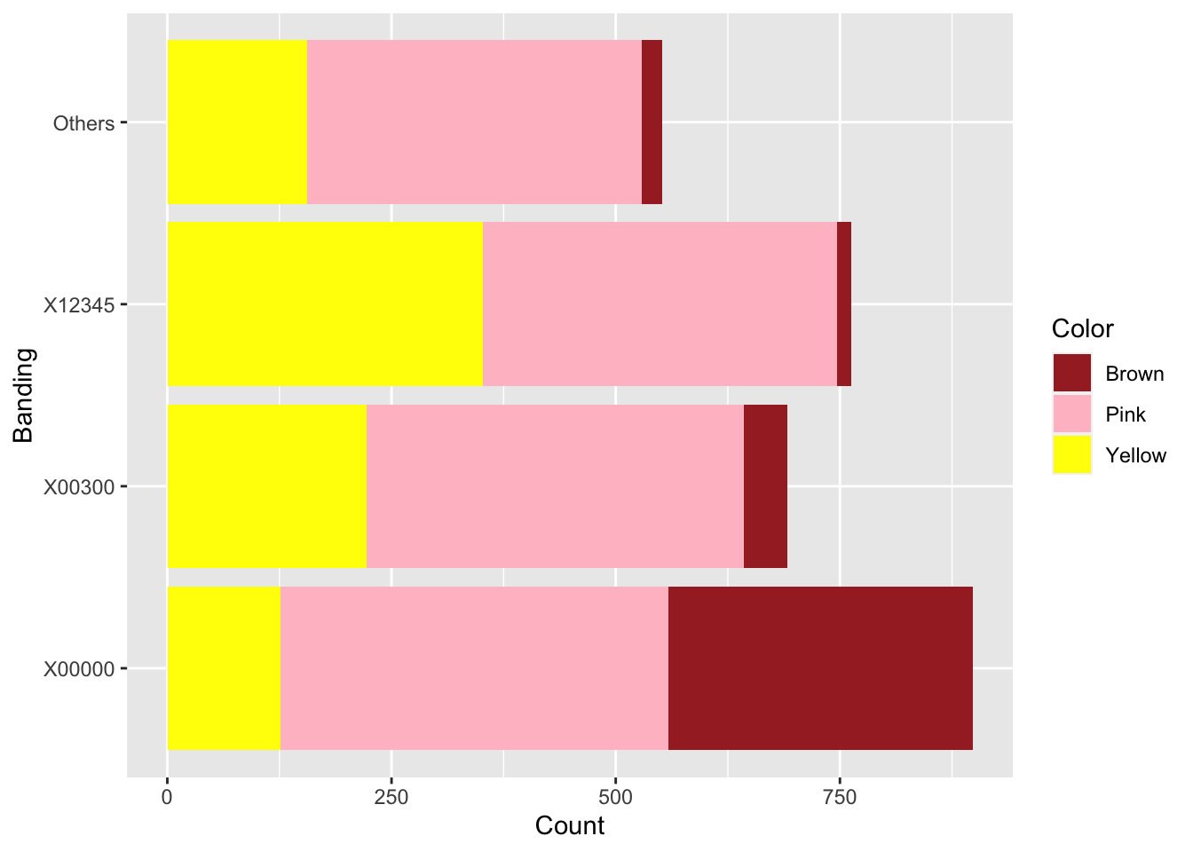

Figure 10.1: Snail color and banding.

A common approach to visualizing categorical variables is with a pie chart. Pie charts are out of favor among data scientists because colors are hard to distinguish and the sizes of wedges are difficult to compare visually. In fact, ggplot2 does not include a built-in pie chart geometry. Instead, one applies polar coordinates to a barplot. Here is an example showing the proportions of snails found in each habitat:

snails %>%
  group_by(Habitat) %>%
  summarize(Count = sum(Count)) %>%
  ggplot(aes(x = NA, y = Count, fill = Habitat)) +
  geom_bar(stat = "identity") +
  coord_polar("y") +
  theme_void()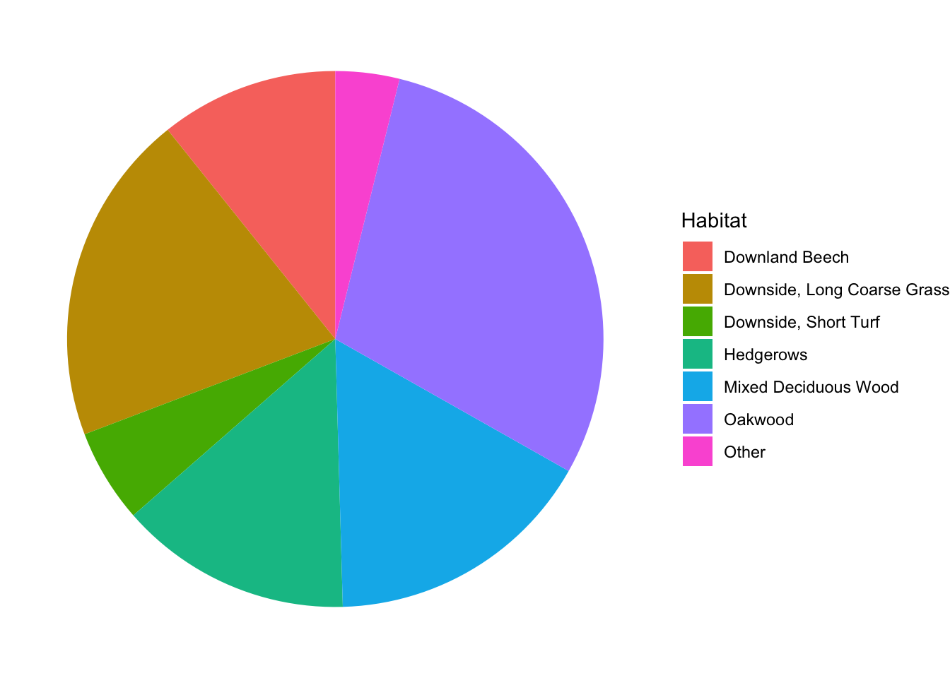

Can you tell whether there were more snails in the Hedgerows or in the Mixed Deciduous Wood? If you have colorblindness or happen to be reading a black and white copy of this text, you probably cannot even tell which wedge is which.

10.2 Inference on a proportion

The simplest setting for categorical data is that of a single binomial random variable. Here \(X \sim \text{Binom}(n,p)\) is a count of successes on \(n\) independent identical trials with probability of success \(p\). A typical experiment would fix a value of \(n\), perform \(n\) Bernoulli trials, and produce a value of \(X\). From this single value of \(X\), we are interested in learning about the unknown population parameter \(p\). For example, we may want to test whether the true proportion of times a die shows a 6 when rolled is actually 1/6. We might choose to toss the die \(n = 1000\) times and count the number of times \(X\) that a 6 occurs.

Polling is an important application. Before an election, a polling organization will sample likely voters and ask them whether they prefer a particular candidate. The results of the poll should give an estimate for the true proportion of voters \(p\) who prefer that candidate. The case of a voter poll is not formally a Bernoulli trial unless you allow the possibility of asking the same person twice; however, if the population is large then polling approximates a Bernoulli trial well enough to use these methods.

If \(X\) is the number of successes on \(n\) trials, the point estimate for the true proportion \(p\) is given by \[ \hat p = \frac{X}{n} \]

Recall that \(E[\hat{p}] = \frac 1nE[X] = \frac{1}{n}np = p\), so \(\hat{p}\) is an unbiased estimate of \(p\). The standard deviation \(\sigma(\hat{p})\) is \(\sqrt{p(1-p)/n}\), so that a larger sample size \(n\) will lead to less variation in \(\hat{p}\) and therefore a better estimate of \(p\).

Our goal is to use the sample statistic \(\hat{p}\) to calculate confidence intervals and perform hypothesis testing with regards to \(p\).

This section introduces one sample tests of proportions. Here, we present the theory associated with performing exact binomial hypothesis tests using binom.test, as well as prop.test, which uses the normal approximation.

A one sample test of proportions requires a hypothesized value of \(p_0\). Often \(p_0 = 0.5\), meaning we expect success and failure to be equally likely outcomes of the Bernoulli trial. Or, \(p_0\) may come from historic values or a known larger population. The hypotheses are:

\[ H_0: p = p_0; \qquad H_a: p \not= p_0\]

You run \(n\) trials and obtain \(x\) successes, so your estimate for \(p\) is given by \(\hat p = x/n\). (We are thinking of \(x\) as data rather than as a random variable.) Presumably, \(\hat p\) is not exactly equal to \(p_0\), and you wish to determine the probability of obtaining an estimate that unlikely or more unlikely, assuming \(H_0\) is true.

10.2.1 Exact binomial test

Our first approach is the binomial test, which is an exact test in that it calculates a \(p\)-value using probabilities coming from the binomial distribution.

For the \(p\)-value, we are going to add the probabilities of all outcomes that are no more likely than the outcome that was obtained, since if we are going to reject when we obtain \(x\) successes, we would also reject if we obtain a number of successes that was even less likely to occur. Formally, the \(p\)-value for the exact binomial test is given by:

\[ \sum_{y:\ P(X = y) \leq P(X = x)} P(X=y)\]

Example 10.1

Consider the wrist data. Approximately 10.6% of the world’s population is left-handed⁷⁹. Is this sample of elderly Finns consistent with the proportion of left-handers in the world? In this binomial random variable, we choose left-handedness as success. Then \(p\) is the true proportion of elderly Finns who are left-handed and \(p_0 = 0.106\). Our hypotheses are:

\[ H_0: p = 0.106; \qquad H_a: p \not= 0.106 \]

The sample contains 104 observations and has 7 left-handed patients, giving \(\hat{p} = 7/104 \approx 0.067\), which is lower than \(p_0\). The probability of getting exactly 7 successes under \(H_0\) is dbinom(7, 104, 0.106), or 0.061. Anything less than 7 successes is less likely under the null hypothesis, so we would add all of those to get part of the \(p\)-value. To determine which values we add for successes greater than 7, we look for all outcomes that have probability of occurring (under the null hypothesis) less than 0.061. That is all outcomes 15 through 104, since \(X = 14\) is more likely than \(X = 7\) (dbinom(14, 104, 0.106) = 0.075 > 0.061) while \(X = 15\) is less likely than \(X = 7\) (dbinom(15, 104, 0.106) = 0.053 < 0.061).

The calculation is illustrated in Figure 10.2, where the dashed red line indicates the probability of observing exactly 7 successes. We sum all of the probabilities that are at or below the dashed red line.

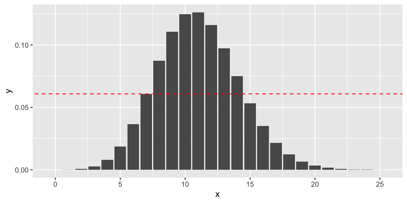
Figure 10.2: The pmf for \(X \sim \text{Binom}(104, 0.106)\), with a line at \(P(X = 7)\). \(X\) values past 25 are negligible and not shown.

The \(p\)-value is \[ P(X \le 7) + P(X \ge 15) \] where \(X\sim \text{Binom}(n = 104, p = 0.106)\).

sum(dbinom(x = 0:7, size = 104, prob = 0.106)) +
  sum(dbinom(x = 15:104, size = 104, prob = 0.106))

## [1] 0.2628259

R will make these computations for us, naturally, in the following way.

binom.test(x = 7, n = 104, p = 0.106)

## 
##  Exact binomial test
## 
## data:  7 and 104
## number of successes = 7, number of trials = 104, p-value =
## 0.2628
## alternative hypothesis: true probability of success is not equal to 0.106
## 95 percent confidence interval:
##  0.02748752 0.13377135
## sample estimates:
## probability of success 
##             0.06730769

With a \(p\)-value of 0.26, we fail to reject the null hypothesis. There is not sufficient evidence to conclude that elderly Finns have a different proportion of left-handers than the world’s proportion of lefties.

The binom.test function also produces the 95% confidence interval for \(p\). In this example, we are 95% confident that the true proportion of left-handed elderly Finns is in the interval \([0.027, 0.134]\). Since \(0.106\) lies in the 95% confidence interval, we failed to reject the null hypothesis at the \(\alpha = 0.05\) level.

10.2.2 One sample test of proportions

When \(n\) is large and \(p\) isn’t too close to 0 or 1, binomial random variables with \(n\) trials and probability of success \(p\) are well approximated by normal random variables with mean \(np\) and standard deviation \(\sqrt{np(1 - p)}\). This can be used to get approximate \(p\)-values associated with the hypothesis test \(H_0: p = p_0\) versus \(H_a: p\not= p_0\).

As before, we need to compute the probability under \(H_0\) of obtaining an outcome that is as likely or less likely than obtaining \(x\) successes. However, in this case we are using the normal approximation, which is symmetric about its mean. The \(p\)-value is twice the area of the tail outside of \(x\).

The prop.test function performs this calculation, and has identical syntax to binom.test.

Example 10.2

We return to the wrist example, testing \(H_0: p = 0.106\) versus \(H_a: p\not= 0.106\). Let \(X\) be a binomial random variable with \(n = 104\) and \(p = 0.106\). \(X\) is approximated by a normal variable \(Y\) with \[\begin{align} \mu(Y) &= np = 104 \cdot 0.106 = 11.024\\ \sigma(Y) &= \sqrt{np(1 - p)} = \sqrt{104 \cdot 0.106 \cdot 0.894} = 3.13934. \end{align}\]

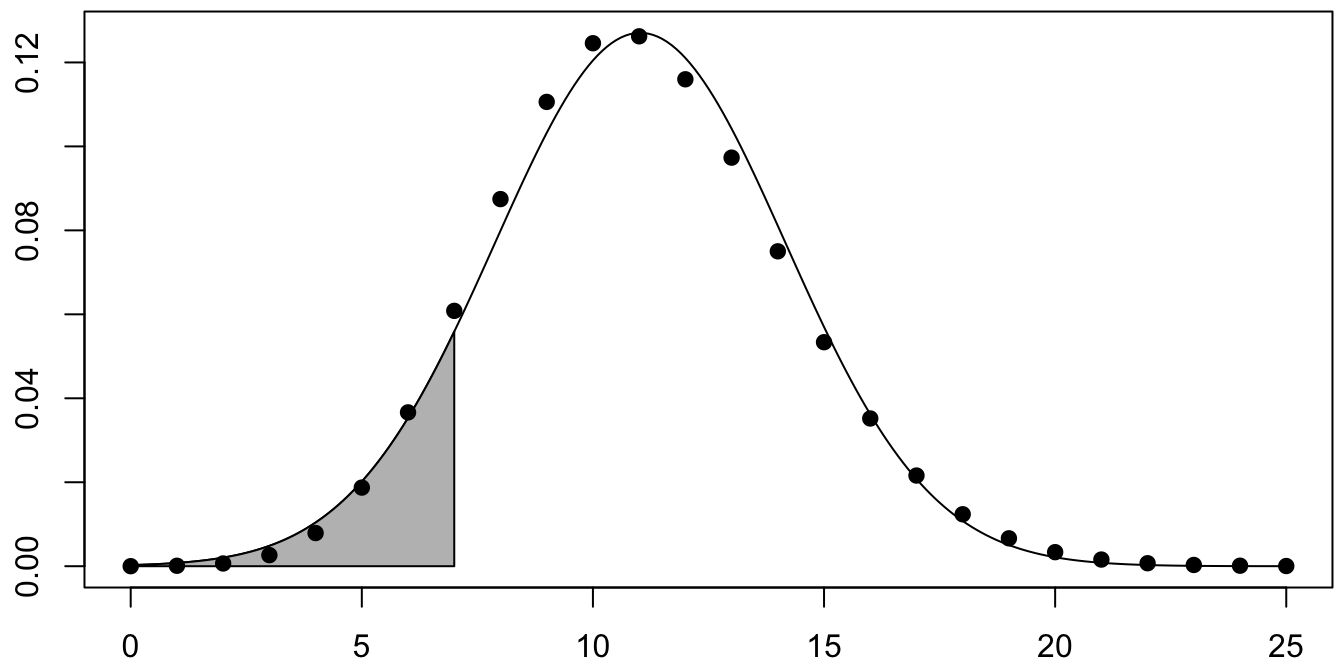
Figure 10.3: Binomial rv with normal approximation overlaid.

Figure 10.3 is a plot of the pmf of \(X\) with its normal approximation \(Y\) overlaid. The shaded area corresponds to \(Y \leq 7\). The \(p\)-value is twice that area, which we compute with pnorm:

2 * pnorm(7, 11.024, 3.13934)

## [1] 0.1999135

For a better approximation, we perform a continuity correction (see also Example 4.26). The basic idea is that \(Y\) is a continuous rv, so when \(Y = 7.3\), for example, we need to decide what integer value that should be associated with. Rounding suggests that \(Y=7.3\) should correspond to \(X=7\) and be included in the shaded area. The continuity correction includes values from 7 to 7.5 in the \(p\)-value, resulting in a corrected \(p\)-value of:

2 * pnorm(7.5, 11.024, 3.13934)

## [1] 0.2616376

The continuity correction gives a more accurate approximation to the underlying binomial rv, but not necessarily a closer approximation to the exact binomial test.

The built-in R function for the one sample test of proportions is prop.test:

prop.test(x = 7, n = 104, p = 0.106)$p.value

## [1] 0.2616376

The prop.test function performs continuity correction by default. The \(p\)-value here is almost identical to the result of binom.test, and as before we fail to reject \(H_0\). The confidence interval produced is also quite similar to the exact binomial test.

Tryit 10.1

Look at the full output of prop.test(x = 7, n = 104, p = 0.106), and observe that the test statistic is given as a \(\chi^2\) random variable with 1 degree of freedom. Confirm that the test statistic is \(c = \left((\tilde x - np_0)/\sqrt{np_0(1 - p_0)}\right)^2\), where \(\tilde x\) is the number of successes after a continuity correction (in this case, \(\tilde x = 7.5\)).

Use pchisq(c, 1, lower.tail = FALSE) to recompute the \(p\)-value using this test statistic. You should get the same answer \(p=\) 0.2616377.

Example 10.3

The Economist/YouGov Poll leading up to the 2016 presidential election sampled 3669 likely voters and found that 1798 intended to vote for Clinton. Assuming that this is a random sample from all likely voters, find a 99% confidence interval for \(p\), the true proportion of likely voters who intended to vote for Clinton at the time of the poll.

prop.test(x = 1798, n = 3699, conf.level = 0.99)$conf.int

## [1] 0.4648186 0.5073862
## attr(,"conf.level")
## [1] 0.99

We are 99% confident that the true proportion of likely Clinton voters was between .465 and .507. In fact, 48.2% of voters did vote for Clinton, and the true value does fall in the 99% confidence interval range.

Most polls do not report a confidence interval. Typically, they report the point estimator \(\hat{p}\) and the margin of error, which is half the width of the 95% confidence interval. For this poll, \(\hat{p} \approx 0.486\) and the 95% confidence interval is \([0.470, 0.502]\) so the pollsters would report that they found 48.6% in favor of Clinton with a margin of error of 1.6%.

10.3 \(\chi^2\) tests

The \(\chi^2\) test is a general approach to testing the hypothesis that tabular data follows a given distribution. It relies on the Central Limit Theorem, in that the various counts in the tabular data are assumed to be approximately normally distributed.

The setting for \(\chi^2\) testing requires tabular data. For each cell in the table, the count of observations that fall in that cell is a random variable. We denote the observed counts in the \(k\) cells by \(X_1, \dotsc, X_k\). The null hypothesis requires an expected count for each cell, \(E[X_i]\). The test statistic is the \(\chi^2\) statistic.

Definition 10.4

If \(X_1, \dotsc, X_k\) are the observed counts of cells in tabular data, then the \(\chi^2\) statistic is:

\[ \chi^2 = \sum_{i=1}^k \frac{(X_i - E[X_i])^2}{E[X_i]} \]

The \(\chi^2\) statistic is always positive, and will be larger when the observed values \(X_i\) are far from the expected values \(E[X_i]\). In all cases we consider, the \(\chi^2\) statistic will have approximately the \(\chi^2\) distribution with \(d\) degrees of freedom, for some \(d < k\). The \(p\)-value for the test is the probability of a \(\chi^2\) value as large or larger than the observed \(\chi^2\). The R function chisq.test computes \(\chi^2\) and the corresponding \(p\)-value.

The \(\chi^2\) test is always a one-tailed test. For example, if we observe \(\chi^2 = 10\) and have four degrees of freedom, the \(p\)-value corresponds to the shaded area in Figure 10.4.

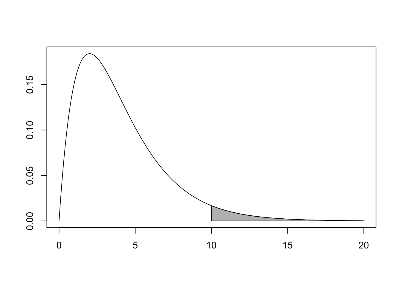
Figure 10.4: \(\chi^2\) distribution with \(p\)-value shaded.

The full theory behind the \(\chi^2\) test is beyond the scope of this book, but in the remainder of this section we give some motivation for the formula for \(\chi^2\) and the meaning of degrees of freedom. A reader less interested in theory could proceed to Section 10.3.1.

Consider the value in one particular cell of tabular data. For each of the \(n\) observations in the sample, the observation either lies in the cell or it does not, hence the count in that one cell can be considered as a binomial rv \(X_i\). Let \(p_i\) be the probability a random observation is in that cell. Then \(E[X_i] = np_i\) and \(\sigma(X_i) = \sqrt{np_i(1-p_i)}\). If \(np_i\) is sufficiently large (at least 5, say) then \(X_i\) is approximately normal and \[ \frac{X_i - np_i}{\sqrt{np_i(1-p_i)}} \sim Z_i, \] where \(Z_i\) is a standard normal variable. Squaring both sides and multiplying by \((1-p_i)\) we have \[ (1-p_i)Z_i^2 \sim \frac{(X_i - np_i)^2}{np_i} = \frac{(X_i - E[X_i])^2}{E[X_i]} \]

As long as all cell counts are large enough, the \(\chi^2\) statistic is approximately \[ \chi^2 = \sum_{i=1}^k (1-p_i)Z_i^2 \] In this expression, the \(Z_i\) are standard normal but not independent random variables. In many circumstances, one can rewrite these \(k\) variables in terms of a smaller number \(d\) of independent standard normal rvs and find that the \(\chi^2\) statistic does have a \(\chi^2\) distribution with \(d\) degrees of freedom. The details of this process require some advanced linear algebra and making precise what we mean when we say \(X_i\) are approximately normal. The details of the dependence are not hard to work out in the simplest case when the table has two cells.

Example 10.5

Consider a table with two cells, with \(n\) observations, cell probabilities \(p_1\), \(p_2\), and cell counts given by the random variables \(X_1\) and \(X_2\):

\[ \begin{array}{|c|c|} \hline X_1 & X_2 \\ \hline \end{array} \]

This is simply a single binomial rv in disguise, with \(X_1\) the count of successes and \(X_2\) the count of failures. In particular, \(p_1 + p_2 = 1\) and \(X_1 + X_2 = n\). Notice that

\[ \frac{X_1 - np_1}{\sqrt{np_1(1-p_1)}} + \frac{X_2 - np_2}{\sqrt{np_2(1-p_2)}} = \frac{X_1 + X_2 - n(p_1 + p_2)}{\sqrt{np_1p_2}} = \frac{n - n(1)}{\sqrt{np_1p_2}} = 0. \]

So the two variables \(Z_1\) and \(Z_2\) are not independent, and satisfy the equation \(Z_1 + Z_2 = 0\). Then both can be written in terms of a single rv \(Z\) with \(Z_1 = Z\) and \(Z_2 = -Z\). As long as \(X_1\) and \(X_2\) are both large, \(Z_i\) will be approximately standard normal, and \[ \chi^2 = (1-p_1)Z_1^2 + (1-p_2)Z_2^2 = (1- p_1 + 1 - p_2)Z^2 = Z^2. \] We see that \(\chi^2\) has the \(\chi^2\) distribution with one df.

The table in this example has two entries, giving two possible counts \(X_1\) and \(X_2\). The constraint that these counts must sum to \(n\) leaves only the single degree of freedom to choose \(X_1\).

10.3.1 \(\chi^2\) test for given probabilities

In this section, we consider data coming from a single categorical variable, typically displayed in a \(1 \times k\) table:

\[ \begin{array}{|c|c|c|c|} \hline X_1 & X_2 & \quad\dotsb\quad & X_k \\ \hline \end{array} \]

For our null hypothesis, we take some vector of probabilities \(p_1, \dotsc, p_k\) as given. Because there are \(k\) cells to fill and a single constraint (the cells sum to \(n\)), the \(\chi^2\) statistic will have \(k-1\) df.

The most common case is when we assume all cells are equally likely, in which case this approach is called the \(\chi^2\) test for uniformity.

Example 10.6

Doyle, Bottomley, and Angell⁸⁰ investigated the “Relative Age Effect,” the disadvantage of being the youngest in a cohort relative to being the oldest. The difference in outcomes can persist for years beyond any difference in actual ability relative to age difference.

In this study, the authors found the number of boys enrolled in the British elite soccer academies for under 18 years of age. They binned the boys into three age groups: oldest, middle, and youngest, with approximately 1/3 of all British children in each group. The number of boys in the elite soccer academies was:

\[ \begin{array}{|c|c|c|} \hline \text{Oldest} & \text{Middle} & \text{Youngest} \\ \hline 631 & 321 & 155 \\ \hline \end{array} \]

The null hypothesis is that the boys should be equally distributed among the three groups, or equivalently \(H_0: p_i = \frac{1}{3}\). There are a total of 1107 boys in this study. Under the null hypothesis, we expect \(369 = 1107/3\) in each group. Then \[ \chi^2 = \frac{(631-369)^2}{369} + \frac{(321-369)^2}{369} + \frac{(155-369)^2}{369} \approx 316.38. \] The test statistic \(\chi^2\) has the \(\chi^2\) distribution with \(2 = 3-1\) degrees of freedom, and a quick glance at that distribution shows that our observed 316.38 is impossibly unlikely to occur by chance. The \(p\)-value is essentially 0, and we reject the null hypothesis. Boys’ ages in elite British soccer academies are not uniformly distributed across the three age bands for a given year.

In R, the computation is done with chisq.test:

boys <- c(631, 321, 155)
chisq.test(boys, p = c(1 / 3, 1 / 3, 1 / 3))

## 
##  Chi-squared test for given probabilities
## 
## data:  boys
## X-squared = 316.38, df = 2, p-value < 2.2e-16

Example 10.7

Benford’s Law is used in forensic accounting to detect falsified or manufactured data. When data, such as financial or economic data, occurs over several orders of magnitude, the first digits of the values follow the distribution

\[ P(\text{first digit is}~d) = \log_{10}(1 + 1/d) \]

benford <- log10(1 + 1 / (1:9))
round(benford, 2)

## [1] 0.30 0.18 0.12 0.10 0.08 0.07 0.06 0.05 0.05

The data fosdata::rio_instagram has the number of Instagram followers for gold medal winners at the 2016 Olympics. First, we extract the first digits of each athlete’s number of followers:

rio <- fosdata::rio_instagram %>%
  mutate(first_digit = stringr::str_extract(n_follower, "[0-9]")) %>%
  filter(!is.na(first_digit))

Let’s visually compare the counts of observed first digits (as bars) to the expected counts from Benford’s Law (red dots):

rio %>% ggplot(aes(x = first_digit)) +
  geom_bar() +
  geom_point(
    data = data.frame(x = 1:9, y = benford * nrow(rio)),
    aes(x, y), color = "red", size = 5
  )

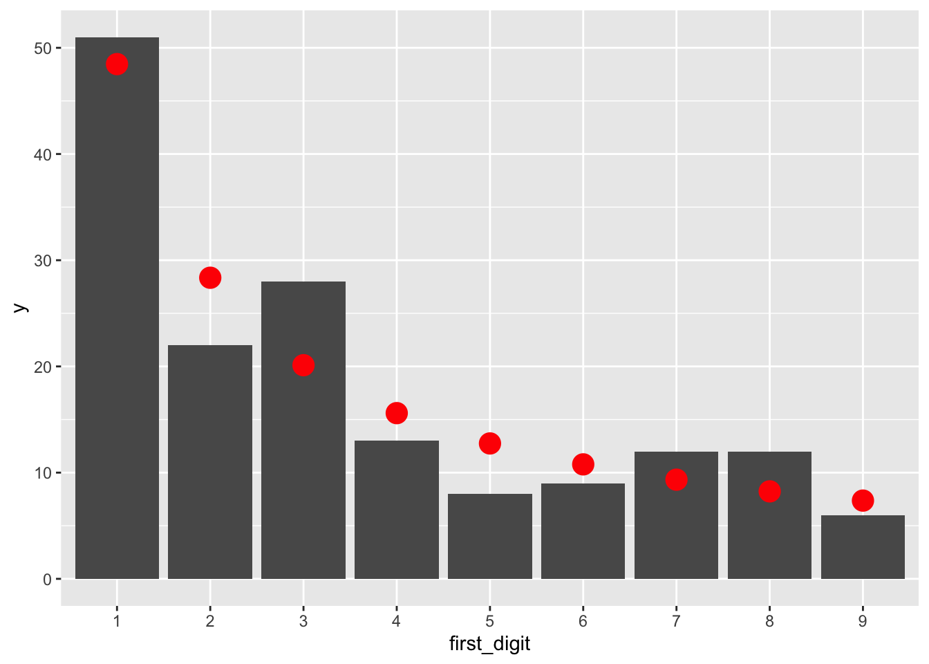
Is the observed data consistent with Benford’s Law?

chisq.test(table(rio$first_digit), p = benford)

## 
##  Chi-squared test for given probabilities
## 
## data:  table(rio$first_digit)
## X-squared = 9.876, df = 8, p-value = 0.2738

The observed value of \(\chi^2\) is 9.876, from a \(\chi^2\) distribution with \(8 = 9 - 1\) degrees of freedom. This is not extraordinary. The \(p\)-value is 0.2738 and we fail to reject \(H_0\). The data is consistent with Benford’s Law.

10.4 \(\chi^2\) goodness of fit

In this section, we consider tabular data that is hypothesized to follow a parametric model. When the parameters of the model are estimated from the observed data, the model fits the data better than it should. Each estimated parameter reduces the degrees of freedom in the \(\chi^2\) distribution by one.

When testing goodness of fit, the \(\chi^2\) statistic is approximately \(\chi^2\) with degrees of freedom given by the following:

\[ \text{degrees of freedom} = \text{bins} - 1 - \text{parameters estimated from the data}. \]

We will explore this claim through simulation in Section 10.4.1.

Example 10.8

Goals in a soccer game arrive at random moments and could be reasonably modeled by a Poisson process. If so, the total number of goals scored in a soccer game should be a Poisson rv.

The data set world_cup from fosdata contains the results of the 2014 and 2015 FIFA World Cup soccer finals. Let’s get the number of goals scored by each team in each game of the 2015 finals:

goals <- fosdata::world_cup %>%
  filter(competition == "2015 FIFA Women's World Cup") %>%
  tidyr::pivot_longer(cols = contains("score"), values_to = "score") %>%
  pull(score) # pull extracts the "score" column as a vector
table(goals)

## goals
##  0  1  2  3  4  5  6 10 
## 30 40 20  6  3  2  1  2

We want to perform a hypothesis test to determine whether a Poisson model is a good fit for the distribution of goals scored. The Poisson distribution has one parameter, the rate \(\lambda\). The expected value of a Poisson rv is \(\lambda\), so we estimate \(\lambda\) from the data:

lambda <- mean(goals)

Here \(\lambda \approx 1.4\), meaning 1.4 goals were scored per game, on average. Figure 10.5 displays the observed counts of goals with the expected counts from the Poisson model \(\text{Pois}(\lambda)\) in red.

Figure 10.5: Goals scored by each team in each game of the 2015 World Cup. Poisson model shown with red dots.

Since the \(\chi^2\) test relies on the Central Limit Theorem, each cell in the table should have a large expected value to be approximately normal. Traditionally, the threshold is that a cell’s expected count should be at least five. Here, all cells with 4 or more goals are too small. The solution is to bin these small counts into one category, giving five total categories: zero goals, one goal, two goals, three goals, or 4+ goals. The observed and expected counts for the five categories are:

expected_goals <- 104 * c(
  dpois(0:3, lambda),
  ppois(3, lambda, lower.tail = FALSE)
)
observed_goals <- c(30, 40, 20, 6, 8)

Goals	0	1	2	3	4+
Observed	30	40	20	6	8
Expected	25.5	35.9	25.2	11.8	5.6

The \(\chi^2\) test statistic will have \(3 = 5 - 1 - 1\) df, since:

• There are 5 bins.
• The bins sum to 104, losing one df.
• The model’s one parameter \(\lambda\) was estimated from the data, losing one df.

We compute the \(\chi^2\) test statistic and \(p\)-value manually, because the chisq.test function is unaware that our expected values were modeled from the data, and would use the incorrect df.

chi_2 <- sum((observed_goals - expected_goals)^2 / expected_goals)
chi_2

## [1] 6.147538

pchisq(chi_2, df = 3, lower.tail = FALSE)

## [1] 0.1046487

The observed value of \(\chi^2\) is 6.15. The \(p\)-value of this test is 0.105, and we would not reject \(H_0\) at the \(\alpha = .05\) level. This test does not give evidence against goal scoring being Poisson.

Note that there is one aspect of this data that is highly unlikely under the assumption that the data comes from a Poisson random variable: ten goals were scored on two different occasions. The \(\chi^2\) test did not consider that, because we binned those large values into a single category. If you believe that data might not be Poisson because you suspect it will have unusually large values (rather than unusually many large values), then the \(\chi^2\) test will not be very powerful.

10.4.1 Simulations

This section investigates the test statistic in the \(\chi^2\) goodness of fit test via simulation. We observe that it does follow the \(\chi^2\) distribution with df equal to bins minus one minus number of parameters estimated from the data.

Suppose that data comes from a Poisson variable \(X\) with mean 2 and there are \(N = 200\) data points.

test_data <- rpois(200, 2)
table(test_data)

## test_data
##  0  1  2  3  4  5  6  7 
## 24 53 54 35 19 12  2  1

The expected count in bin 5 is 200 * dpois(5,2) which is 7.2, large enough to use. The expected count in bin 6 is only 2.4, so we combine all bins 5 and higher. In a real experiment, the sample data could affect the number of bins chosen, but we ignore that technicality.

test_data[test_data > 5] <- 5
table(test_data)

## test_data
##  0  1  2  3  4  5 
## 24 53 54 35 19 15

Next, compute the expected counts for each bin using the rate \(\lambda\) estimated from the data. Bins 0-4 can use dpois but bin 5 needs the entire tail of the Poisson distribution.

lambda <- mean(test_data)
p_fit <- c(dpois(0:4, lambda), ppois(4, lambda, lower.tail = FALSE))
expected <- 200 * p_fit

Finally, we produce one value of the test statistic:

observed <- table(test_data)
sum((observed - expected)^2 / expected)

## [1] 0.9263996

Naively using chisq.test with the data and the fit probabilities gives the same value of \(\chi^2 = 0.9264\), but produces a \(p\)-value using 5 df, which is wrong. The function does not know that we used one df to estimate a parameter.

# wrong df produces incorrect p-value
chisq.test(observed, p = p_fit)

## 
##  Chi-squared test for given probabilities
## 
## data:  observed
## X-squared = 0.9264, df = 5, p-value = 0.9683

We now replicate to produce a sample of values of the test statistic to verify that 4 is the correct df for this test:

sim_data <- replicate(10000, {
  test_data <- rpois(200, 2) # produce data
  test_data[test_data > 5] <- 5 # re-bin to six bins
  observed <- table(test_data)

  lambda <- mean(test_data)
  expected <- 200 * c(
    dpois(0:4, lambda),
    ppois(4, lambda, lower.tail = FALSE)
  )

  sum((observed - expected)^2 / expected)
})

plot(density(sim_data),
  main = "Test statistic and chi-squared distributions"
)
curve(dchisq(x, 4), add = TRUE, col = "blue")
curve(dchisq(x, 5), add = TRUE, col = "red")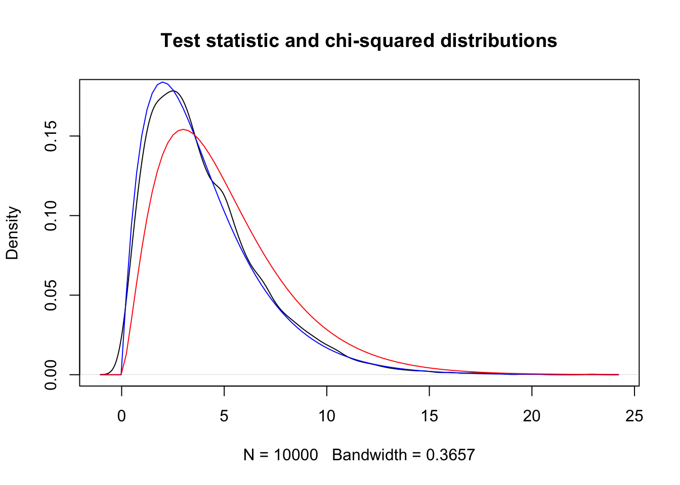

The black curve is the probability density from our simulated data. The blue curve is \(\chi^2\) with 4 degrees of freedom, equal to (bins - parameters - 1). The red curve is \(\chi^2\) with 5 degrees of freedom and does not match the observations. This seems to be pretty compelling.

10.5 \(\chi^2\) tests on cross tables

Given two categorical variables \(A\) and \(B\), we can form a cross table with one cell for each pair of values \((A_i,B_j)\). That cell’s count is a random variable \(X_{ij}\):

\[ \begin{array}{c|c|c|c|c|} & B_1 & B_2 & \quad\dotsb\quad & B_n \\ \hline A_1 & X_{11} & X_{12} & \quad\dotsb\quad & X_{1n} \\ \hline A_2 & X_{21} & X_{22} & \quad\dotsb\quad & X_{2n} \\ \hline \vdots & \vdots &\vdots & \quad\ddots\quad & \vdots \\ \hline A_m & X_{m1} & X_{m2} & \quad\dotsb\quad & X_{mn} \\ \hline \end{array} \]

As in all \(\chi^2\) tests, the null hypothesis leads to an expected value for each cell. In this setting, we require a probability \(p_{ij}\) that an observation lies in cell \((i,j)\), \(p_{ij} = P(A = A_i\ \cap\ B = B_j)\). These probabilities are called the joint probability distribution of \(A\) and \(B\).

The hypothesized joint probability distribution needs to come from somewhere. It could come from historical or population data, or by fitting a parametric model, in which case the methods of the previous two sections apply.

We assume that \(B\) is random (and perhaps \(A\) as well, but not necessarily) and we consider the null hypothesis that the probability distribution of \(B\) is independent of the levels of \(A\). Let \(N\) be the total number of observations. If we let \(a_i = \frac{1}{N} \sum_j X_{ij}\) denote the proportion of observations for which \(A = A_i\) and \(b_j = \frac{1}{N} \sum_i X_{ij}\) denote the proportion of responses for which \(B = B_j\), then under the assumption of \(H_0\) we would hypothesize that \[ p_{ij} = a_i b_j. \] It follows that \(E[X_{ij}] = N a_i b_j\).

The test statistic is \[ \chi^2 = \sum_{i,j} \frac{(X_{ij} - E[X_{ij}])^2}{E[X_{ij}]}. \]

When the expected cell counts \(E[X_{ij}]\) are all large enough, the test statistic has approximately a \(\chi^2\) distribution with \((\text{columns} - 1)(\text{rows} - 1)\) degrees of freedom. There are two explanations for why this is the correct degrees of freedom, depending on the details of the experimental design. The mechanics of the test itself, however, do not depend on the experimental design. Sections 10.5.1 and 10.5.2 discuss the details.

10.5.1 \(\chi^2\) test of independence

In the \(\chi^2\) test of independence, the levels of \(A\) and \(B\) are both random. In this case, we are testing

\[ H_0: A {\text{ and }} B {\text{ are independent random variables}} \]
versus the alternative that they are not independent. The values of \(p_{ij} = a_i b_j\) have a natural interpretation as \(p_{ij} = P(A = A_i \cap B = B_j) = P(A = A_i) P(B = B_j)\).

To understand the degrees of freedom in the test for independence, the experimental design matters. We fix \(N\) the total number of observations, and for each subject the two categorical variables \(A\) and \(B\) are measured (see Example 10.9). The row and column marginal sums of the cross table are random. Then:

• There are \(mn\) cells.
• There are \(m + n\) marginal probabilities \(a_i\) and \(b_j\) estimated from the data, and \(\sum a_i = \sum b_i = 1\), so we lose \(m + n - 2\) df.
• All cell counts must add to \(N\), losing one df.
• \(mn - (m + n - 2) - 1 = (m - 1)(n - 1)\)

Example 10.9

Are grove snail color and banding patterns related? Figure 10.1 suggests that brown snails are more likely to be unbanded than the other colors.

In R, the \(\chi^2\) test for independence is simple: we pass the cross table to chisq.test.

snailtable <- xtabs(Count ~ Color + Banding, data = fosdata::snails)
snailtable

##         Banding
## Color    X00000 X00300 X12345 Others
##   Brown     339     48     16     23
##   Pink      433    421    395    373
##   Yellow    126    222    352    156

chisq.test(snailtable)

## 
##  Pearson's Chi-squared test
## 
## data:  snailtable
## X-squared = 652.77, df = 6, p-value < 2.2e-16

The cross table is \(3 \times 4\), so the \(\chi^2\) statistic has \((3-1)(4-1) = 6\) df. The \(p\)-value is very small, so we reject \(H_0\). Snail color and banding are not independent.

Let’s reproduce the results of chisq.test. First, compute marginal probabilities.

a_color <- snailtable %>%
  marginSums(margin = 1) %>%
  proportions()
a_color
b_band <- snailtable %>%
  marginSums(margin = 2) %>%
  proportions()
b_band

## Color
##     Brown      Pink    Yellow 
## 0.1466942 0.5585399 0.2947658

## Banding
##    X00000    X00300    X12345    Others 
## 0.3092287 0.2379477 0.2627410 0.1900826

Next, compute the joint distribution \(p_{ij} = a_ib_j\). This uses the matrix multiplication operator %*% and the matrix transpose t to compute all 12 entries at once. The result is multiplied by \(N = 2904\) to get expected cell counts:

p_joint <- a_color %*% t(b_band)
expected <- p_joint * 2904
round(expected, 1)

##         Banding
## Color    X00000 X00300 X12345 Others
##   Brown   131.7  101.4  111.9   81.0
##   Pink    501.6  386.0  426.2  308.3
##   Yellow  264.7  203.7  224.9  162.7

Finally, compute the \(\chi^2\) test statistic and the \(p\)-value, which match the results of chisq.test.

chi2 <- sum((snailtable - expected)^2 / expected)
chi2

## [1] 652.7671

pchisq(chi2, df = 6, lower.tail = FALSE)

## [1] 9.605329e-138

It is instructive to view each cell’s contribution to \(\chi^2\) graphically as a “heatmap” to provide a sense of which cells were most responsible for the dependence between color and banding.

((snailtable - expected)^2 / expected) %>%
  as.data.frame() %>%
  ggplot(aes(x = Banding, y = Color, fill = Freq)) +
  geom_tile() +
  scale_fill_gradient(low = "white", high = "red")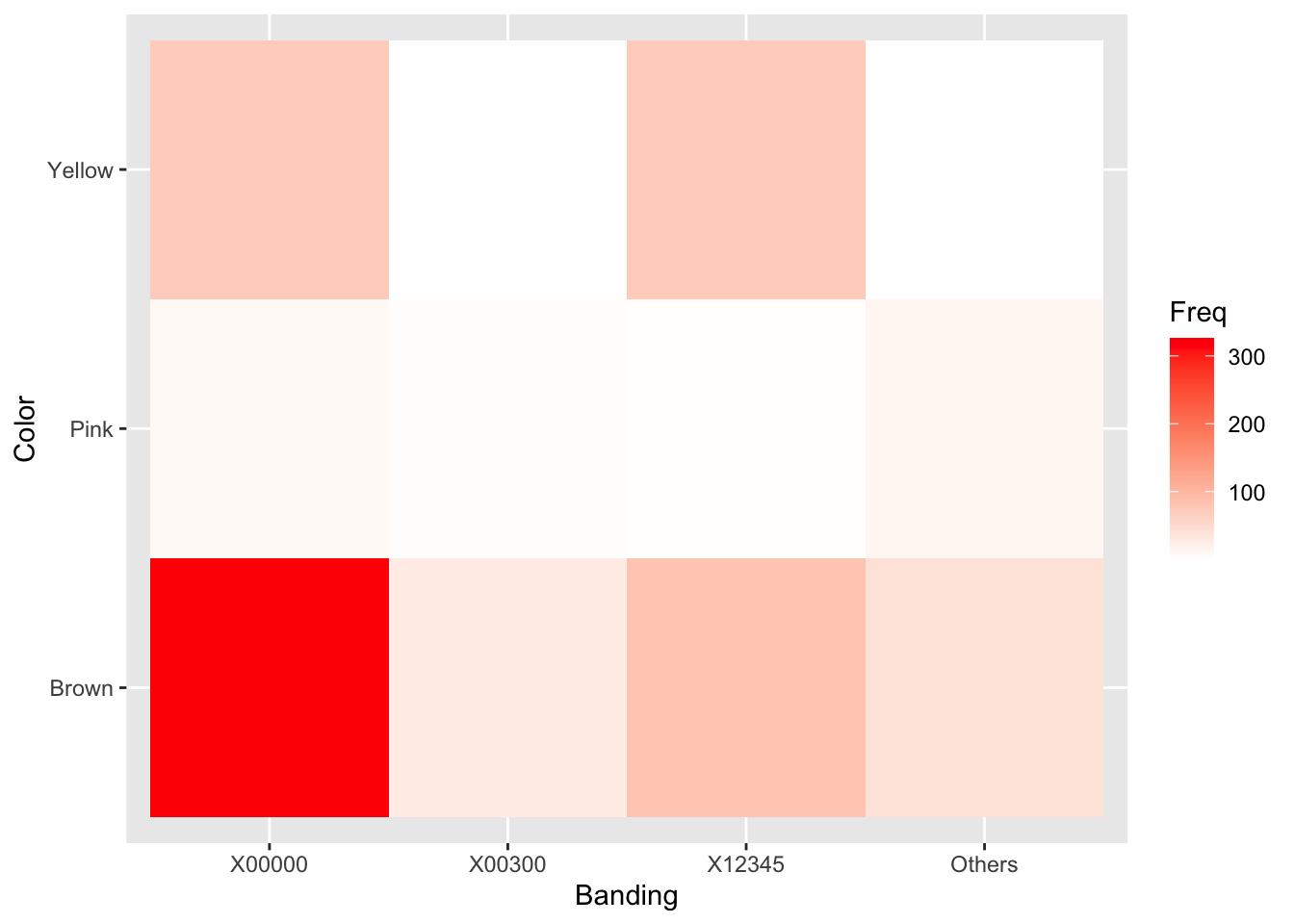

Clearly, most of the interaction between Banding and Color comes from the overabundance of unbanded (X00000) Brown snails. The authors of the original study were interested in environmental effects on color and bandedness of snails. It is possible, though a more thorough analysis would be required, that an environment that favors the survival of brown snails also favors unbanded snails.

Example 10.10

To what extent do animals display conformity? That is, will they forgo personal information in order to follow the majority? Researchers⁸¹ studied conformity among dogs. They trained a subject dog to walk around a wall in one direction in order to receive a treat. After training, the subject dog then watched other dogs walk around the wall in the opposite direction. If the subject dog changes its behavior to match the dogs it observed, it is evidence of conforming behavior.

The data from this experiment is available as the dogs data frame in the fosdata package.

dogs <- fosdata::dogs

This data set has quite a bit going on. In particular, each dog repeated the experiment three times, which means that it would be unwise to assume independence across trials. So, we will restrict to the first trial only. We also restrict to dogs that did not drop out of the experiment.

dogs_trial1 <- filter(dogs, trial == 1, dropout == 0)

Subject dogs participated under three conditions. The control group (condition = 0) observed no other dogs, and was simply asked to repeat what they were trained to do. Another group (condition = 1) saw one dog that went the “wrong” way around the wall three times. Another group (condition = 3) saw three different dogs that each went the wrong way around the wall one time.

We summarize the results of the experiment with a table showing the three experimental conditions in the three rows and whether the subject dog conformed or not in the two columns.

xtabs(~ condition + conform, data = dogs_trial1)

##          conform
## condition  0  1
##         0 12  3
##         1 20  9
##         3 17  9

The null hypothesis is that conform and condition are independent variables, so that the three groups of dogs would have the same conforming behavior. We store the cross table and apply the \(\chi^2\) test for independence:

dogtable <- xtabs(~ condition + conform, data = dogs_trial1)
chisq.test(dogtable)

## Warning in chisq.test(dogtable): Chi-squared approximation may be
## incorrect

## 
##  Pearson's Chi-squared test
## 
## data:  dogtable
## X-squared = 0.9928, df = 2, p-value = 0.6087

The \(p\)-value is 0.61, so there is not significant evidence that the conform and condition variables are dependent. Dogs do not disobey training to conform, at least according to this simple analysis.

The \(\chi^2\) test reports 2 df because we have 3 rows and 2 columns, and \((3-1)(2-1) = 2\). The test also produces a warning, because the expected cell count for conforming dogs under condition 0 is low. With a high \(p\)-value and good cell counts elsewhere, the lack of accuracy is not a concern.

Tryit 10.2

A link to the paper associated with the dogs data is given in ?fosdata::dogs. Find the place in the paper where they perform the above \(\chi^2\) test, and read the authors’ explanation related to it.

10.5.2 \(\chi^2\) test of homogeneity

In a \(\chi^2\) test of homogeneity, one of the variables \(A\) and \(B\) is not random. For example, if an experimenter decides to collect data on cats by finding 100 American shorthair cats, 100 highlander cats, and 100 munchkin cats and measuring eye color for each of the 300 cats, then the number of cats of each breed is not a random variable. A test of this type is called a \(\chi^2\) test of homogeneity, or a \(\chi^2\) test with one fixed margin. However, we are still interested in whether the distribution of eye color depends on the breed of the cat, and we proceed exactly in the same manner as before, with a slightly reworded null hypothesis and a different justification of the degrees of freedom. We denote \(B\) as the variable that is random. Our null hypothesis is:

\[ H_0: {\text{ the distribution of $B$ does not depend on the level of $A$}} \] and the alternative hypothesis is that the distribution of \(B\) does depend on the level of \(A\). We compute degrees of freedom as follows:

• There are \(mn\) cells.
• There are \(n\) marginal probabilities \(b_1, \ldots, b_n\). Since these must sum to 1, we lose \(n - 1\) degrees of freedom.
• Each row sums to a fixed number, so we lose \(m\) degrees of freedom.
• We do not lose any degrees of freedom for all bins summing to \(N\), since that is implied by the column condition.
• Total degrees of freedom are \(mn - (n - 1) - m = (m - 1)(n - 1)\), as in the case of the \(\chi^2\) test of independence.

The mechanics of a \(\chi^2\) test of homogeneity are the same as a \(\chi^2\) test of independence.

Example 10.11

Consider the sharks data set⁸² in the fosdata package. Participants were paid 25 cents to listen to either silence, ominous music, or uplifting music while possibly watching a video on sharks. An equal number were recruited for each type of music. They were then asked to give their rating from 1-7 on their willingness to help conserve endangered sharks. We are interested in whether the distribution of the participants’ willingness to conserve sharks depends on the type of music they listened to.

We start by computing the cross table of the data.

sharks <- fosdata::sharks
shark_tabs <- xtabs(~ music + conserve, data = sharks)
shark_tabs %>%
  addmargins()

##            conserve
## music         1   2   3   4   5   6   7 Sum
##   ominous    10   6  13  28  43  49  54 203
##   silence     5   6  12  28  57  51  48 207
##   uplifting   6   6   7  24  59  44  60 206
##   Sum        21  18  32  80 159 144 162 616

The rows do not add up to exactly the same number because some participants dropped out of the study. We ignore this problem and continue.

chisq.test(shark_tabs)

## 
##  Pearson's Chi-squared test
## 
## data:  shark_tabs
## X-squared = 9.0547, df = 12, p-value = 0.6982

We see that there is not sufficient evidence to conclude that the distribution of willingness to help conserve endangered sharks depends on the type of music heard (\(p = .6982\)).

10.5.3 Two sample test for equality of proportions

An important special case of the \(\chi^2\) test for independence is the two sample test for equality of proportions.

Suppose that \(n_1\) trials are made from population 1 with \(x_1\) successes, and that \(n_2\) trials are made from population 2 with \(x_2\) successes. We wish to test \(H_0: p_1 = p_2\) versus \(H_a: p_1 \not= p_2\), where \(p_i\) is the true probability of success from population \(i\). We create a \(2\times 2\) table of values as follows:

\[ \begin{array}{c|c|c|} & \text{Pop. 1} & \text{Pop. 2} \\ \hline \text{Successes} & x_{1} & x_{2} \\ \hline \text{Failures} & n_1 - x_1 & n_2 - x_2 \\ \hline \end{array} \]

The null hypothesis says that \(p_1 = p_2\). We estimate this common probability using all the data:

\[ \hat{p} = \frac{\text{Successes}}{\text{Trials}} = \frac{x_1 + x_2}{n_1 + n_2} \]

The expected number of successes under \(H_0\) is calculated from \(n_1\), \(n_2\), and \(\hat{p}\):

\[ \begin{array}{c|c|c|} & \text{Pop. 1} & \text{Pop. 2} \\ \hline \text{Exp. Successes} & n_1\hat{p} & n_2\hat{p} \\ \hline \text{Exp. Failures} & n_1(1-\hat{p}) & n_2(1-\hat{p})\\ \hline \end{array} \]

We then compute the \(\chi^2\) test statistic. This has 1 df, since there were 4 cells, two constraints that the columns sum to \(n_1\), \(n_2\), and one parameter estimated from the data.

The test statistic and \(p\)-value can be computed with chisq.test. The prop.test function performs the same computation, and allows for finer control over the test in this specific setting.

Example 10.12

Researchers randomly assigned patients with wrist fractures to receive a cast in one of two positions, the VFUDC position and the functional position. The assignment of cast position should be independent of which wrist (left or right) was fractured. We produce a cross table from the data in fosdata::wrist and run the \(\chi^2\) test for independence:

wrist_table <- xtabs(~ cast_position + fracture_side, data = fosdata::wrist)
wrist_table

##              fracture_side
## cast_position  1  2
##             1 18 32
##             2 27 28

chisq.test(wrist_table)

## 
##  Pearson's Chi-squared test with Yates' continuity correction
## 
## data:  wrist_table
## X-squared = 1.3372, df = 1, p-value = 0.2475

For prop.test we need to know the group sizes, \(n_1 = 45\) with right-side fractures and \(n_2 = 60\) with left-side fractures. We also need the number of successes, which we arbitrarily select as cast position 1.

prop.test(c(18, 32), c(45, 60))

## 
##  2-sample test for equality of proportions with continuity
##  correction
## 
## data:  c(18, 32) out of c(45, 60)
## X-squared = 1.3372, df = 1, p-value = 0.2475
## alternative hypothesis: two.sided
## 95 percent confidence interval:
##  -0.34362515  0.07695849
## sample estimates:
##    prop 1    prop 2 
## 0.4000000 0.5333333

The prop.test function applies a continuity correction by default. chisq.test only applies continuity correction in this \(2 \times 2\) case. There seems to be some disagreement on whether or not continuity correction is desirable. From the point of view of this text, we would choose the version that has observed type I error rate closest to the assigned rate of \(\alpha\). Let’s run some simulations, using \(n_1 = 45\), \(n_2 = 60\), and success probability \(p = 50/105\) to match the wrist example.

p <- 50 / 105
n1 <- 45
n2 <- 60
data_ccorrected <- replicate(10000, {
  x1 <- rbinom(1, n1, p)
  x2 <- rbinom(1, n2, p)
  prop.test(c(x1, x2), c(n1, n2), correct = TRUE)$p.value
})
data_not_ccorrected <- replicate(10000, {
  x1 <- rbinom(1, n1, p)
  x2 <- rbinom(1, n2, p)
  prop.test(c(x1, x2), c(n1, n2), correct = FALSE)$p.value
})

mean(data_ccorrected < .05)

## [1] 0.0284

mean(data_not_ccorrected < .05)

## [1] 0.0529

We see that for this sample size and common probability of success, correct = FALSE comes closer to the desired type I error rate of 0.05, but is a bit too high. This holds across a wide range of \(p\), \(n_1\) and \(n_2\). Using continuity correction tends to have effective error rates lower than the designed type I error rates, while correct = FALSE has type I error rates closer to the designed type I error rates.

Example 10.13

Consider the babynames data set in the babynames package. Is there a statistically significant difference in the proportion of girls named “Bella”⁸³ in 2007 and the proportion of girls named “Bella” in 2009?

We will need to do some data wrangling on this data and define a binomial variable bella:

bella_table <- babynames::babynames %>%
  filter(sex == "F", year %in% c(2007, 2009)) %>%
  mutate(name = ifelse(name == "Bella", "Bella", "Not Bella")) %>%
  xtabs(n ~ year + name, data = .)
bella_table

##       name
## year     Bella Not Bella
##   2007    2253   1918366
##   2009    4532   1830067

We see that the number of girls named “Bella” nearly doubled from 2007 to 2009. The two sample proportions test shows that this was highly significant.

prop.test(bella_table)$p.value

## [1] 2.982331e-192

10.6 Exact and Monte Carlo methods

The \(\chi^2\) methods of the previous sections all approximate discrete variables with continuous (normal) variables. Exact and Monte Carlo methods are very general approaches to testing tabular data, and neither method requires assumptions of normality.

Exact methods produce exact \(p\)-values by examining all possible ways the \(N\) outcomes could fill the table. The first step of an exact method is to compute the test statistic associated to the observed data, often \(\chi^2\). Then for each possible table, compute the test statistic and the probability of that table occurring, assuming the null hypothesis. The \(p\)-value is the sum of the probabilities of the tables whose associated test statistics are as extreme or more extreme than the observed test statistic. This \(p\)-value is exact because (assuming the null hypothesis) it is exactly the probability of obtaining a test statistic as or more extreme than the one coming from the data.

Unfortunately, the number of ways to fill out a table grows exponentially with the number of cells in the table (or more precisely, exponentially in the degrees of freedom). This makes exact methods unreasonably slow when \(N\) is large or the table has many cells. Monte Carlo methods present a compromise that avoids assumptions but stays computationally tractable. Rather than investigate every possible way to fill the table, we randomly create many tables according to the null hypothesis. For each, the \(\chi^2\) statistic is computed. The \(p\)-value is taken to be the proportion of generated tables that have a larger \(\chi^2\) statistic than the observed data. Though we compute the \(\chi^2\) statistic for the observed and simulated tables, we do not rely on assumptions about its distribution – it may not have a \(\chi^2\) distribution at all.

Example 10.14

Return to the data on age cohorts in soccer, introduced in Example 10.6. There were three relative age groups in each cohort year: old, middle, and young. Our null hypothesis is that each age group should be equally likely for an elite soccer player in a given cohort. The data has \(N = 1107\) boys, with 631, 321, and 155 in the old, middle, and young groups.

To apply Monte Carlo methods, we need to generate simulated \(3\times 1\) tables. We use the R function rmultinom, which generates multinomially distributed random number vectors. As with all random variable generation functions in R, the first argument to rmultinom is the number of simulations we want. Then there are two required parameters, the number of observations \(N\) in each table and the null hypothesis probability distribution. Here are ten tables that might result from the experiment, one in each column.

sim_boys <- rmultinom(10, size = 1107, prob = c(1 / 3, 1 / 3, 1 / 3))
sim_boys

##      [,1] [,2] [,3] [,4] [,5] [,6] [,7] [,8] [,9] [,10]
## [1,]  355  337  373  357  412  387  370  364  378   410
## [2,]  394  367  383  368  362  366  364  374  387   348
## [3,]  358  403  351  382  333  354  373  369  342   349

From the first column, one possible outcome of the soccer study would be to find 355, 394, and 358 boys in the old, medium, and young groups. The next nine columns are also possible outcomes, each with \(N = 1107\) observations. It is apparent that the observed value of 631 boys in the “old” group is exceptionally large under \(H_0\).

To get a \(p\)-value, we first compute the \(\chi^2\) statistic for the observed data:

observed_boys <- c(631, 321, 155)
expected_boys <- c(1 / 3, 1 / 3, 1 / 3) * sum(observed_boys)
sum((observed_boys - expected_boys)^2 / expected_boys)

## [1] 316.3794

The \(\chi^2\) statistic is a measure of how far our observed group sizes are from the expected group sizes. For the observed boys, \(\chi^2\) is 316.3794. Next compute the \(\chi^2\) statistic for each set of simulated group sizes:

colSums((sim_boys - expected_boys)^2 / expected_boys)

##  [1] 2.5528455 5.9186992 1.4525745 0.8509485 8.6558266 1.5121951
##  [7] 0.1138211 0.1355014 3.0731707 6.8346883

Again, it is clear that the observed data is quite different than the data that was simulated under \(H_0\). We should use more than 10 simulations, of course, but for this particular data you will never see a value as large as 316 in the simulations. The true \(p\)-value for this experiment is essentially zero.

R can carry out the Monte Carlo method within the chisq.test function:

chisq.test(observed_boys,
  p = c(1 / 3, 1 / 3, 1 / 3),
  simulate.p.value = TRUE
)

## 
##  Chi-squared test for given probabilities with simulated p-value
##  (based on 2000 replicates)
## 
## data:  observed_boys
## X-squared = 316.38, df = NA, p-value = 0.0004998

The function performed 2000 simulations and none of them had a higher \(\chi^2\) value than the observed data. The \(p\)-value was reported as 1/2001, because R always includes the actual data set in addition to the 2000 simulated values. This is a common technique that makes a relatively small absolute difference in estimates.

Example 10.15

Continuing with the boys elite soccer age data, we show how to apply the exact multinomial test.

The idea of the exact test is to sum the probabilities of all tables that lead to test statistics that are as extreme or more extreme than the observed test statistic. The table of boys is \(3 \times 1\), and we need the three values in the table to sum to 1107. In Exercise 10.29, you are asked to show that there are 614386 possible ways to fill a \(3 \times 1\) table with numbers that sum to 1107.

The multinomial.test function in the EMT package carries out this process.

EMT::multinomial.test(observed_boys, prob = c(1 / 3, 1 / 3, 1 / 3))

## 
##  The model includes 614386 different events.
## 
##  The chosen number of trials is rather low, should be at least 10 times the number of possible configurations.
## 
## 
##  Exact Multinomial Test
## 
##     Events        pObs     p.value
##     614386 5.82402e-73 1.97583e-05

As before, the \(p\)-value is 0. The EMT::multinomial.test function can also run Monte Carlo tests using the parameter MonteCarlo = TRUE.

Vignette: Tables

Tables are an often overlooked part of data visualization and presentation. They can also be difficult to do well! In this vignette, we introduce the knitr::kable function, which produces tables compatible with .pdf, .docx and .html output inside of your R Markdown documents.

To make a table using knitr::kable, create a data frame and apply kable to it.

knitr::kable(xtabs(Count ~ Banding + Color, data = snails))

	Brown	Pink	Yellow
X00000	339	433	126
X00300	48	421	222
X12345	16	395	352
Others	23	373	156

Example 10.16

Suppose you are studying the palmerpenguins::penguins data set, and you want to report the mean, standard deviation, range, and number of samples of bill length in each species type. The dplyr package helps to produce the data frame, and we use kable options to create a caption and better column headings. The table is displayed as Table 10.1.

penguins <- palmerpenguins::penguins
penguin_table <- penguins %>%
  filter(!is.na(bill_length_mm)) %>%
  group_by(species) %>%
  summarize(
    mean(bill_length_mm),
    sd(bill_length_mm),
    paste(min(bill_length_mm), max(bill_length_mm), sep = " - "),
    n()
  )
knitr::kable(penguin_table,
  caption = "Bill lengths (mm) for penguins.",
  col.names = c("Species", "Mean", "SD", "Range", "# Birds"),
  digits = 2
)

Table 10.1: Bill lengths (mm) for penguins.

Species	Mean	SD	Range	# Birds
Adelie	38.79	2.66	32.1 – 46	151
Chinstrap	48.83	3.34	40.9 – 58	68
Gentoo	47.50	3.08	40.9 – 59.6	123

The kable package provides only basic table styles. To adjust the width and other features of table style, use the kableExtra package.

Another interesting use of tables is in combination with broom::tidy, which converts the outputs of many common statistical tests into data frames. Let’s see how it works with t.test.

Example 10.17

Display the results of a \(t\)-test of the body temperature data from fosdata::normtemp in a table.

t.test(fosdata::normtemp$temp, mu = 98.6) %>%
  broom::tidy() %>%
  select(1:6) %>%
  knitr::kable(digits = 3)

estimate	statistic	p.value	parameter	conf.low	conf.high
98.249	-5.455	0	129	98.122	98.376

We selected only the first six variables so that the table would better fit the page.

Example 10.18

As a final example, let’s test groups of cars from mtcars to see if their mean mpg is different from 25. The groups we want are the four possible combinations of transmission (am) and engine (vs). This requires four \(t\)-tests, and could be a huge hassle! But, check this out:

mtcars %>%
  group_by(am, vs) %>%
  do(broom::tidy(t.test(.$mpg, mu = 25))) %>%
  select(1:8) %>%
  knitr::kable(
    align = "r", digits = 4,
    caption = "Is mean mpg 25 for combinations of trans and engine?
               A two-sided one sample $t$-test."
  )

Table 10.2: Is mean mpg 25 for combinations of trans and engine? A two-sided one sample \(t\)-test.

am	vs	estimate	statistic	p.value	parameter	conf.low	conf.high
0	0	15.0500	-12.4235	0.0000	11	13.2872	16.8128
0	1	20.7429	-4.5581	0.0039	6	18.4575	23.0282
1	0	19.7500	-3.2078	0.0238	5	15.5430	23.9570
1	1	28.3714	1.8748	0.1099	6	23.9713	32.7716

Exercises

---

Exercises 10.1 – 10.2 require material through Section 10.1.

10.1 Kahle, Sharon, and Baram-Tsabari⁸⁴ examined the reaction to posts to social media by The European Organization for Nuclear Research, better known as CERN. The data is available in the cern data frame in the fosdata package. Recreate the content of the table that appeared in their paper using xtabs and addmargins. To get the order of the levels the same, you will need to change the levels of the factor in the data set.

Image credit: Kahle et al..Image Credit
Kahle et al.. This is an open access article distributed under the terms of the Creative Commons Attribution License. https://journals.plos.org/plosone/article?id=10.1371/journal.pone.0156409

10.2

Consider the cern data set in the fosdata package. Create a figure similar to Figure 10.1 which illustrates the total number of likes for each type of post, colored by the platform. French Twitter may not show up because it has so few likes.

---

Exercises 10.3 – 10.8 require material through Section 10.2.

10.3

Suppose you are testing \(H_0: p = 0.4\) versus \(H_a: p \not= 0.4\). You collect 20 pieces of data and observe 12 successes. Use dbinom to compute the \(p\)-value associated with the exact binomial test, and check using binom.test.

10.4

Suppose you are testing \(H_0: p = 0.4\) versus \(H_a: p \not= 0.4\). You collect 100 pieces of data and observe 33 successes. Use the normal approximation to the binomial to find an approximate \(p\)-value associated with the hypothesis test.

10.5

Shaquille O’Neal (Shaq) was an NBA basketball player from 1992–2011. He was a notoriously bad free throw shooter⁸⁵. Shaq always claimed, however, that the true probability of him making a free throw was greater than 50%. Throughout his career, Shaq made 5,935 out of 11,252 free throws attempted. Is there sufficient evidence to conclude that Shaq indeed had a better than 50/50 chance of making a free throw?

10.6

Diaconis, Holmes and Montgomery⁸⁶ claim that vigorously flipped coins tend to come up the same way they started. In a real coin tossing experiment⁸⁷, two UC Berkeley students tossed coins a total of 40 thousand times in order to assess whether this is true. Out of the 40,000 tosses, 20,245 landed on the same side as they were tossed from.

1. Find a (two-sided) 99% confidence interval for \(p\), the true proportion of times a coin will land on the same side it is tossed from.
2. Clearly state the null and alternative hypotheses, defining any parameters that you use.
3. Is there sufficient evidence to reject the null hypothesis at the \(\alpha = .05\) level based on this experiment? What is the \(p\)-value?

10.7

This exercise requires material from Section 6.7 or knowledge of loops. The curious case of the dishonest statistician – suppose a statistician wants to “prove” that a coin is not a fair coin. They decide to start flipping the coin, and after 10 tosses they will run a hypothesis test on \(H_0: p = 1/2\) versus \(H_a: p \not= 1/2\). If they reject at the \(\alpha = .05\) level, they stop. Otherwise, they toss the coin one more time and run the test again. They repeatedly toss and run the test until either they reject \(H_0\) or they toss the coin 100 times (hey, they’re dishonest and lazy). Estimate using simulation the probability that the dishonest statistician will reject \(H_0\).

10.8 (Hard)

Suppose you wish to test whether a die truly comes up “6” 1/6 of the time. You decide to roll the die until you observe 100 sixes. You do this, and it takes 560 rolls to observe 100 sixes.

1. State the appropriate null and alternative hypotheses.
2. Explain why prop.test and binom.test are not formally valid to do a hypothesis test.
3. Use reasoning similar to that in the explanation of binom.test above and the function dnbinom to compute a \(p\)-value.
4. Should you accept or reject the null hypothesis?

---

Exercises 10.9 – 10.12 require material through Section 10.3.

10.9

Suppose you are collecting categorical data that comes in three levels. You wish to test whether the levels are equally likely using a \(\chi^2\) test. You collect 150 items and obtain a test statistic of 4.32. What is the \(p\)-value associated with this experiment?

10.10

Recall that the colors of M&M’s supposedly follow this distribution:

\[ \begin{array}{cccccc} Yellow & Red & Orange & Brown & Green & Blue \\ 0.14 & 0.13 & 0.20 & 0.12 & 0.20 & 0.21 \end{array} \]

Imagine you bought 10,000 M&M’s and got the following color counts:

\[ \begin{array}{cccccc} Yellow & Red & Orange & Brown & Green & Blue \\ 1357 & 1321 & 1946 & 1182 & 2052 & 2142 \end{array} \]

Does your sample appear to follow the known color distribution? Perform the appropriate \(\chi^2\) test at the \(\alpha = .05\) level and interpret.

10.11

The data set fosdata::bechdel has information on budget and earnings for many popular movies.

1. Is the budget data consistent with Benford’s Law?
2. Is the intgross data consistent with Benford’s Law?
3. Is the domgross data consistent with Benford’s Law? (Hint: one movie had no domestic gross. Bonus: which one was it?)

10.12

The United States Census Bureau produces estimates of population for all cities and towns in the U.S. On the census website http://www.census.gov, find population estimates for all incorporated places (cities and towns) for any one state. Import that data into R. Do the values for city and town population numbers follow Benford’s Law? Report your results with a plot and a \(p\)-value as in Example 10.7.

---

Exercises 10.13 – 10.17 require material through Section 10.4.

10.13

Did the goals scored by each team in each game of the 2014 FIFA Men’s World Cup soccer final follow a Poisson distribution? Perform a \(\chi^2\) goodness of fit test at the \(\alpha = 0.05\) level, binning values 4 and above. Data is in fosdata::world_cup.

10.14

Consider the austen data set in the fosdata package. In this exercise, we are testing to see whether the number of times that words are repeated after their first occurrence is Poisson. Restrict to the first chapter of Pride and Prejudice, and count the number of times that each word is repeated, and see that we obtain the following table:

## .
##   0   1   2   3   4   5   6   7   8   9  10  11  12  13  14  16  17  20 
## 201  50  16  13  12   2   5   5   2   1   4   2   1   2   1   2   1   1 
##  21  28  30 
##   1   1   1

Use a \(\chi^2\) goodness of fit test with \(\alpha = .05\) to test whether the distribution of repetitions of words is consistent with a Poisson distribution.

10.15

Powerball is a lottery game in which players try to guess the numbers on six balls drawn randomly. The first five are white balls and the sixth is a special red ball called the powerball. The results of all Powerball drawings from February 2010 to July 2020 are available in fosdata::powerball.

1. Plot the numbers drawn over time. Use color to distinguish the six balls. What do you observe? You will need pivot_longer to tidy the data.
2. Use a \(\chi^2\) test of uniformity to check if all numbers ever drawn fit a uniform distribution.
3. Restrict to draws after October 4, 2015, and only consider the white balls drawn, Ball1-Ball5. Do they fit a uniform distribution?
4. Restrict to draws after October 4, 2015, and only consider Ball1. Check that it is not uniform. Explain why not.

10.16

In this exercise, we explore doing \(\chi^2\) goodness of fit tests for continuous variables. Consider the hdl variable in the adipose data set in fosdata. We wish to test whether the data is normal using a \(\chi^2\) goodness of fit test and 7 bins.

1. Estimate the mean \(\mu\) and the standard deviation \(\sigma\) of the HDL.
2. Use qnorm(seq(0, 1, length.out = 8), mu, sigma) to create the dividing points (breaks) between 7 equally likely regions. The first region is \((-\infty, 0.8988)\).
3. Use table(cut(aa, breaks = breaks)) to obtain the observed distribution of values in bins. The expected number in each bin is the number of data points over 7, since each bin is equally likely.
4. Compute the \(\chi^2\) test statistic as the difference between observed and expected squared, divided by the expected.
5. Compute the probability of getting this test-statistic or larger using pchisq. The degrees of freedom is the number of bins minus 3, one because the sum has to be 71 and the other because you are estimating two parameters from the data.
6. Is there evidence to conclude that HDL is not normally distributed?

10.17

Consider the fosdata::normtemp data set. Use a goodness of fit test with 10 bins, all with equal probabilities, to test the normality of the temperature data set. Note that in this case, you will need to estimate two parameters, so the degrees of freedom will need to be adjusted appropriately.

---

Exercises 10.18 – 10.28 require material through Section 10.5.

10.18

Clark and Westerberg⁸⁸ investigated whether people can learn to toss heads more often than tails. The participants were told to start with a heads up coin, toss the coin from the same height every time, and catch it at the same height, while trying to get the number of revolutions to work out so as to obtain heads. After training, the first participant got 162 heads and 138 tails.

1. Find a 95% confidence interval for \(p\), the proportion of times this participant will get heads.
2. Clearly state the null and alternative hypotheses, defining any parameters.
3. Is there sufficient evidence to reject the null hypothesis at the \(\alpha = .01\) level based on this experiment? What is the \(p\)-value?
4. The second participant got 175 heads and 125 tails. Is there sufficient evidence to conclude that the probability of getting heads is different for the two participants at the \(\alpha = .05\) level?

10.19

Left digit bias is when people attribute a difference to two numbers based on the first digit of the number, when there is not really a large difference between the numbers. In an article⁸⁹, researchers studied left digit bias in the context of treatment choices for patients who were just over or just under 80 years old.

Researchers found that 265 of 5036 patients admitted with acute myocardial infarction who were admitted in the two weeks after their 80th birthday underwent Coronary-Artery Bypass Graft (CABG) surgery, while 308 out of 4426 patients with the same diagnosis admitted in the two weeks before their 80th birthday underwent CABG. There is no recommendation in clinical guidelines to reduce CABG use at the age of 80. Is there a statistically significant difference in the percentage of patients receiving CABG in the two groups?

---

Exercises 10.20 and 10.21 consider the psychology of randomness, as studied in Bar-Hillel et al.⁹⁰

10.20

The researchers considered whether people are good at creating random sequences of heads and tails in a unique way. The researchers recruited 175 people and asked them to create a random sequence of 10 heads and tails, though the researchers were only interested in the first guess. Of the 175 people, 143 predicted heads on the first toss. Let \(p\) be the probability that a randomly selected person will predict heads on the first toss. Perform a hypothesis test of \(p = 0.5\) versus \(p \not= 0.5\) at the \(\alpha = 0.05\) level.

10.21

The researchers also considered whether the linguistic convention of naming heads before tails impacts participants’ choice for their first imaginary coin toss. The authors recruited 54 people and told them to create a sample of size 10 by entering H for heads and T for tails. They recruited 51 people and told them to create a sample of size 10 by entering T for tails and H for heads. A total of 47 of the 54 people in Group 1 chose heads first, while 16 of the 51 people in Group 2 chose heads first. Perform a hypothesis test of \(p_1 = p_2\) versus \(p_1 \not= p_2\) at the \(\alpha = .05\) level, where \(p_i\) is the percentage of heads that people given instructions in Group \(i\) would create as their first guess.

---

10.22

If someone offered you either one really great marble and three mediocre ones, or four mediocre marbles, which would you choose?

Third-grade children in Rijen, the Netherlands, were split into two groups.⁹¹ In group 1, 43 out of 48 children preferred a blue and white striped marble to a solid red marble. In group 2, 12 out of 44 children preferred four solid red marbles to three solid red marbles and one blue and white striped marble. Let \(p_1\) be the proportion of children who would prefer a blue and white marble to a red marble, and let \(p_2\) be the proportion of children who would prefer three red marbles and one blue and white striped marble to four red marbles. Perform a hypothesis test of \(p_1 = p_2\) versus \(p_1 \not= p_2\) at the \(\alpha = .05\) level.

10.23

A 2017 study⁹² considered the care of patients with burns. A patient who stayed in the hospital for seven or more days past the last surgery for a burn is considered an extended postoperative stay. The researchers examined records and found that for patients with scalds, 30 did not have extended stays while 16 did have extended stays. For patients with flame burns, 51 did not have extended stays while 78 did have extended stays. Test whether the proportion of extended stays is the same for scald patients as for flame burn patients at the \(\alpha = .05\) level.

10.24

Ronald Reagan became president of the United States in 1980. The babynames::babynames data set contains information on babies named “Reagan” born in the United States. Is there a statistically significant difference in the percentage of babies (of either sex) named “Reagan” in the United States in 1982 and in 1978? If so, which direction was the change?

10.25

Consider the dogs data set in the fosdata package. For dogs in trial 1 that were shown a single dog going around the wall in the “wrong” direction three times, is there a statistically significant difference in the proportion that stay and the proportion that switch depending on their start direction?

10.26

Consider the sharks data set in the fosdata package. Participants were assigned to listen to either silence, ominous music, or uplifting music while watching a video about sharks. They then ranked sharks on various scales.

1. Create a cross table of the type of music listened to and the response to dangerous; “how well does dangerous describe sharks.”
2. Perform a \(\chi^2\) test of homogeneity to test whether the ranking of how well “dangerous” describes sharks has the same distribution across the type of music heard.

10.27

Police sergeants in the Boston Police Department take an exam for promotion to lieutenant. In 2008, 91 sergeants took the lieutenant promotion test. Of them, 65 were white and 26 were Black or Hispanic.⁹³ The passing rate for white officers was 94%, while the passing rate for minorities was 69%. Was there a significant difference in the passing rates for whites and for minority test takers?

Figure 10.6: Bicycle signage. (Image credit: Hess and Peterson.)

Image credit: Hess and Peterson.Image Credit
Hess and Peterson. This is an open access article distributed under the terms of the Creative Commons Attribution License. https://journals.plos.org/plosone/article?id=10.1371/journal.pone.0136973

10.28

Hess and Peterson⁹⁴ studied whether bicycle signage can affect an automobile driver’s perception of bicycle rights and safety. Load the fosdata::bicycle_signage data, and see the help page for descriptions of the variables.

1. Create a contingency table of the variables bike_move_right2 and treatment.
2. Calculate the proportion of participants who agreed and disagreed for each type of sign treatment. Which sign was most likely to lead participants to disagree?
3. Perform a \(\chi^2\) test of independence on the variables bike_move_right2 and treatment at the \(\alpha = .05\) level. Interpret your answer.

---

Exercise 10.29 requires material through Section 10.6.

10.29

In Example 10.15, we stated that the number of possible ways to fill a \(3 \times 1\) table with non-negative integers that sum to 1107 is 614,386. Explain why this is the case. (Hint: if you know the first two values, then the third one is determined.)

---

76. Raittio et al., “Two Casting Methods Compared in Patients with Colles’ Fracture.”↩︎

77. A J Cain and P M Sheppard, “Selection in the Polymorphic Land Snail Cepæa Nemoralis,” Heredity 4, no. 3 (1950): 275–94.↩︎

78. The R function proportions is new to R 4.0.1 and is recommended as a drop-in replacement for the unfortunately named prop.table.↩︎

79. M Papadatou-Pastou et al., “Human Handedness: A Meta-Analysis.” Psychological Bulletin 146, no. 6 (2020): 481–524, https://doi.org/10.1037/bul0000229.↩︎

80. John R Doyle, Paul A Bottomley, and Rob Angell, “Tails of the Travelling Gaussian Model and the Relative Age Effect: Tales of Age Discrimination and Wasted Talent,” PLOS One 12, no. 4 (April 2017): 1–22, https://doi.org/10.1371/journal.pone.0176206.↩︎

81. Markus Germar et al., “Dogs (Canis Familiaris) Stick to What They Have Learned Rather Than Conform to Their Conspecifics’ Behavior,” PLOS One 13, no. 3 (March 2018): 1–16, https://doi.org/10.1371/journal.pone.0194808.↩︎

82. Andrew P Nosal et al., “The Effect of Background Music in Shark Documentaries on Viewers’ Perceptions of Sharks.” PLOS One 11, no. 8 (2016): e0159279, https://doi.org/10.1371/journal.pone.0159279.↩︎

83. “Bella” was the name of the character played by Kristen Stewart in the movie Twilight, released in 2008. Fun fact, one of the authors has a family member who appeared in The Twilight Saga: Breaking Dawn - Part 2.↩︎

84. Kate Kahle, Aviv J Sharon, and Ayelet Baram-Tsabari, “Footprints of Fascination: Digital Traces of Public Engagement with Particle Physics on CERN’s Social Media Platforms.” PLOS One 11, no. 5 (2016): e0156409.↩︎

85. Shaq is reported to have said, “Me shooting 40 percent at the foul line is just God’s way of saying that nobody’s perfect. If I shot 90 percent from the line, it just wouldn’t be right.”↩︎

86. Persi Diaconis, Susan Holmes, and Richard Montgomery, “Dynamical Bias in the Coin Toss,” SIAM Review 49, no. 2 (2007): 211–35.↩︎

87. Priscilla Ku and Janet Larwood, “40,000 Coin Tosses Yield Ambiguous Evidence for Dynamical Bias,” 2009, https://www.stat.berkeley.edu/~aldous/Real-World/coin_tosses.html.↩︎

88. Matthew P A Clark and Brian D Westerberg, “Holiday Review. How Random Is the Toss of a Coin?” Canadian Medical Association Journal 181, no. 12 (December 2009): E306–8.↩︎

89. Andrew R Olenski et al., “Behavioral Heuristics in Coronary-Artery Bypass Graft Surgery.” N Engl J Med 382, no. 8 (February 2020): 778–79.↩︎

90. M Bar-Hillel, E Peer, and A Acquisti, “‘Heads or Tails?’ – a Reachability Bias in Binary Choice,” Journal of Experimental Psychology: Learning, Memory, and Cognition 40, no. 6 (2014): 1656--1663, https://doi.org/10.1037/xlm0000005.↩︎

91. Ellen R K Evers, Yoel Inbar, and Marcel Zeelenberg, “Set-Fit Effects in Choice.” J Exp Psychol Gen 143, no. 2 (April 2014): 504–9.↩︎

92. Islam Abdelrahman et al., “Division of Overall Duration of Stay into Operative Stay and Postoperative Stay Improves the Overall Estimate as a Measure of Quality of Outcome in Burn Care,” PLOS One 12, no. 3 (March 2017): e0174579–79.↩︎

93. Zack Huffman, “Boston Police Promotion Exam Deemed Biased” (Courthouse News Service, November 18, 2015), https://www.courthousenews.com/boston-police-promotion-exam-deemed-biased/.↩︎

94. George Hess and M Nils Peterson, “"Bicycles May Use Full Lane" Signage Communicates U.S. Roadway Rules and Increases Perception of Safety,” PLOS One 10, no. 8 (August 2015): e0136973.↩︎